
Coursera.org 机器学习 笔记
These are the notes by learning Andrew Ng’s “Machine Learning” from Coursera.org for future review
- Machine Learning
- Machine Learning Algorithms
- Multivariate Linear Regression
- Classification
- Overfitting
- Neural Networks
- To be continued
Machine Learning
- Grew out of work in AI
- New capability for computers
Examples:
Database mining
Large datasets from growth of automation/ web
E.g., Web click data, medical records, biology, engineering
Applications cannot program by hand
E.g., Autonomous helicopter, handwriting recognition, most of Natural Language Processing (NLP), Computer Vision
Self-customizing programs
E.g., Amazon, Netflix product recommendations
Understanding human learning (brain, real AI)
Introduction
- Definition
- Arthur Samuel (1959). Machine Learning: Field of study that gives computers the ability to learn without being explicitly programmed
- Tom Mitchell (1995) Well-posed Leaning Problem: A computer program is said to learn from experience E with respect to some task T and some performance measure P, if its performance on T, as measured by P, improves with experience E.
Machine Learning Algorithms:
Supervised learning
- “Right answers” given
- Regression: Predict continuous valued output
- Classification: Discrete valued output (0 or 1 or others)
Unsupervised learning
- allows us to approach problems with little or no idea what our results should look like.
- We can derive structure from data where we do not necessarily know the effect of the variables.
- We can derive this structure by clustering the data based on relationships among the variables in the data
-
There is no feedback based on the prediction results
- E.g., Organize computing clusters, social network analysis, market segmentation, astronomical data analysis
Model representation
- Notation
- m = Number of training examples
- x’s = “input” variable / features
- y’s = “output” variable / “target” variable
- Hypothesis
- Training set → Learning Algorithm → Hypothesis (h)
- x → h → estimated value of y
- h: X → Y
- h maps x’s to y’s
- Linear regression with one variable or Univariate linear regression
- $ h_{\theta}(x) = \theta_{0} + \theta_{1}x $
- shorthand: $ h(x) $
- $ \theta_{i} $’s: parameters
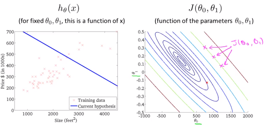
Cost function
- Idea: Choose $ \theta_{0}, \theta_{1} $ so that $ h_{\theta}(x) $ is close to y for our training examples (x,y)
- $ \underset{ \theta_{0}, \ \theta_{1} }{ \mathrm{minimize} } $ $ \dfrac{1}{2m} \displaystyle\sum_{i=1}^m ( \hat{y}^{i}- y^{i} )^2 = $
- $ h_{\theta}(x^{i}) = \theta_{0} + \theta_{1}x^{i} $
- Cost function: $ J(\theta_0, \theta_1) = $
- Octave:
J = 1/(2*m)*sum((X*theta .- y).^2) - also called squared error cost function or squared error function
- Octave:
-
Goal: $ \displaystyle \underset{ \theta_{0}, \ \theta_{1} }{ \mathrm{minimize} } J(\theta_0, \theta_1) $
- contour plots or contour figures:
Gradient descent
- Outline:
- Start with some $ \theta_{0}, \ \theta_{1} $
- Keep changing $ \theta_{0}, \ \theta_{1} $ to reduce $ J(\theta_{0}, \theta_{1}) $ until we hopefully end up at a minimum
- Algorithm
- repeat until convergence { $ \theta_j := \theta_j - \alpha \displaystyle \frac{\partial}{\partial \theta_j} J(\theta_0, \ \theta_1) \ \ (\mathrm{for} \ j = 0 \ \mathrm{and} \ j = 1 ) $ }
- α: learning rate: too small → slow ; too large → overshoot; proper → automatically decrease α over time
- Correct simultaneous update
- temp0 := $ \theta_0 - \alpha \displaystyle \frac{\partial}{\partial \theta_0} J(\theta_0, \ \theta_1) \ \ (\mathrm{for} \ j = 0 \ \mathrm{and} \ j = 1 ) $
- temp1 := $ \theta_1 - \alpha \displaystyle \frac{\partial}{\partial \theta_1} J(\theta_0, \ \theta_1) \ \ (\mathrm{for} \ j = 0 \ \mathrm{and} \ j = 1 ) $
- $ \theta_0 := $ temp0
- $ \theta_1 := $ temp1
- linear regression:
- repeat until convergence:
- $ \theta_0 := \theta_0 - \alpha \frac{1}{m} \sum\limits_{i=1}^{m}(h_\theta(x_{i}) - y_{i}) $
- $ \theta_1 := \theta_1 - \alpha \frac{1}{m} \sum\limits_{i=1}^{m}((h_\theta(x_{i}) - y_{i}) x_{i})$
- Octave:
theta = theta - alpha/m*(X'*(X*theta .- y))
- “Batch” Gradient Descent:
- “Batch”: Each step of gradient descent uses all the training examples
Multivariate Linear Regression
Multiple Features (variables)
- n = number of features
- $ x^{(i)} \text{ for } (i\in { 1,\dots, m } ) $ = input (features) of $ i^{th} $ training examples
- $ x^{i} = [ x_{1}^{i} \ x_{2}^{i} \ \dots \ x_{n}^{i} ]^{T} \in \mathbb{R}^{n} $
- $ x_{j}^{(i)} $ = value of $ j^{th} $ features in $ i^{th} $ training examples
- Hypothesis:
- $ x = [ x_{0} \ x_{1} \ x_{2} \ \dots \ x_{n} ]^{T} \in \mathbb{R}^{n+1} \ \ (x_{0}^{i} = 1) $
- $ \theta = [ \theta_{0} \ \theta_{1} \ \theta_{2} \ \dots \ \theta_{n} ]^{T} \in \mathbb{R}^{n+1} $
- $ h_{\theta}(x) = \theta_{0}x_{0} + \theta_{1}x_{1} + \theta_{2}x_{2} + \dots + \theta_{n}x_{n} \ \ (x_{0} = 1) $
$ \ \ \ \ \ = \theta^{T}x $
- Parameters: $ \theta_{0}, \theta_{1}, \dots , \theta_{n} $
- Cost function: $ J(\theta) = J(\theta_{0}, \theta_{1}, \dots , \theta_{n}) = $
- Gradient descent:
Repeat {
} (simultaneously update for every $ j = 0, \dots, n $ ) -
New algorithm (n ≥ 1):
Repeat {
} (simultaneously update $ \theta_j $ for $ j = 0, \dots, n $ ) - Features Scaling
- Let $ x = \displaystyle \frac{x}{ \mathrm{range} S } $
to get every feature into approximately a $ -1 \leq x \leq 1 $ range - Mean normalization: replace $ x_j \mathrm{with} \frac{x_j - \mu_j}{ s_{j} } $ (Do not apply to $ x_0 = 1 $)
into $ -0.5 \leq x_j \leq 0.5 $ range
- Let $ x = \displaystyle \frac{x}{ \mathrm{range} S } $
- Learning Rate choose
- “Debugging”: plot ( $ \displaystyle\underset{ \theta }{ \mathrm{min} } \ J(\theta) $, No. of iterations)
$ J(\theta) $ should decrease after every iteration → converge (sufficiently α) - Not working → Use smaller α
slow converge → use larger α
- “Debugging”: plot ( $ \displaystyle\underset{ \theta }{ \mathrm{min} } \ J(\theta) $, No. of iterations)
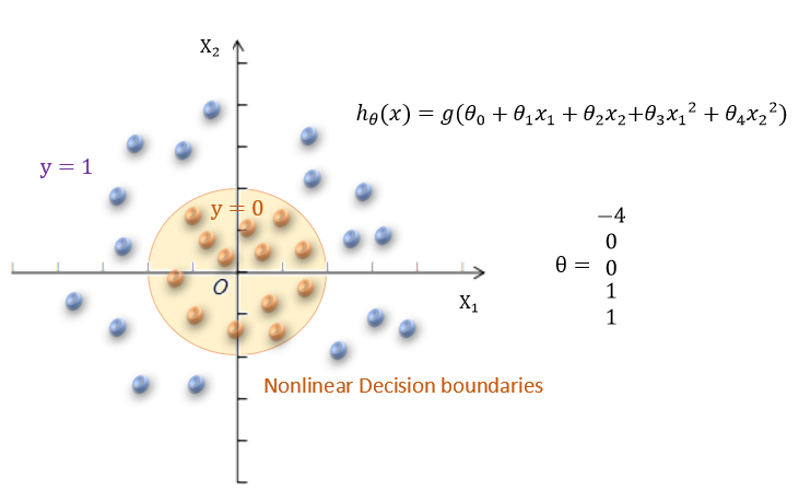
- Create new feature
- Change the behavior or curve of our hypothesis function by making it a quadratic, cubic or square root function or any other form (Features Scaling)
Normal equation
- Definition: Method to solve for θ analytically
- Formula: $ \displaystyle\theta = (X^{T} X)^{-1} X^{T} y $
- Octave:
pinv(x'*x)*x'*y - No need feature scaling
- If n is very large, it works very slow, by compute $ n^3 $
- Octave:
Classification
- Binary classification problem: y = 0 or 1
- Use linear regression:
- To map all predictions greater than 0.5 as a 1 and all less than 0.5 as a 0
- $ h_\theta(x) $ can be >1 or <0, so it does not work well
- Logistic Regression: make $ 0 \le h_\theta(x) \le 1 $
Logistic Regression
- Clasification and Representation
- Sigmoid(Logistic) function: $ g(Z) = \displaystyle\frac{1}{1+e^{-z}} $
- Octave:
h = 1.0 ./ (1.0 + exp(-z)) - $ h_\theta(x) = g(\theta^{T}x) = \displaystyle\frac{1}{1+e^{-\theta^{T}x}} $
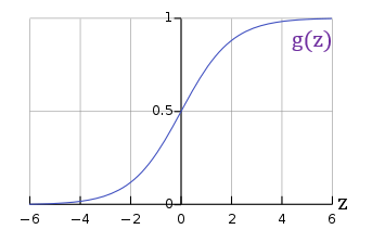
- $ h_\theta(x) = $ estimated probability that y = 1 on input x
- $ h_\theta(x) = P(y=1 \vert x ; \theta) = 1 - P(y=0 \vert x ; \theta) $
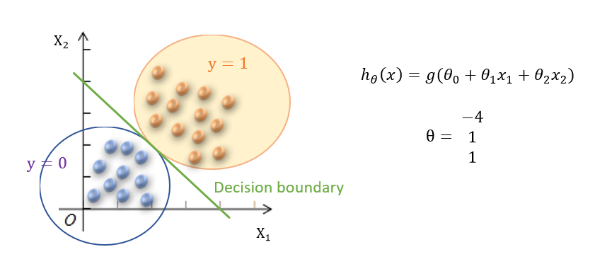
- Decision boundary
- To get discrete 0 or 1 classification, can translate the output of the hypothesis function as:
- $ h_\theta(x) \geq 0.5 \rightarrow y = 1 $
- $ h_\theta(x) \leq 0.5 \rightarrow y = 0 $
- $ g(z) \geq 0.5 $ when $ z \geq 0 $ that $ h_\theta(x) = g(\theta^T x) \geq 0.5 $ when $ \theta^T x \geq 0 $
- From these statements we can say:
- $ \theta^T x \geq 0 \Rightarrow y = 1 $
- $ \theta^T x \leq 0 \Rightarrow y = 0 $
- To get discrete 0 or 1 classification, can translate the output of the hypothesis function as:
- Cost function
- $ J(\theta) = \displaystyle\dfrac{1}{m} \sum_{i=1}^m \mathrm{Cost}(h_\theta(x^{(i)}),y^{(i)}) $
- $ \mathrm{Cost}(h_\theta(x),y) = -\log(h_\theta(x)) $ if y = 1
- $ \mathrm{Cost}(h_\theta(x),y) = -\log(1-h_\theta(x)) $ if y = 0
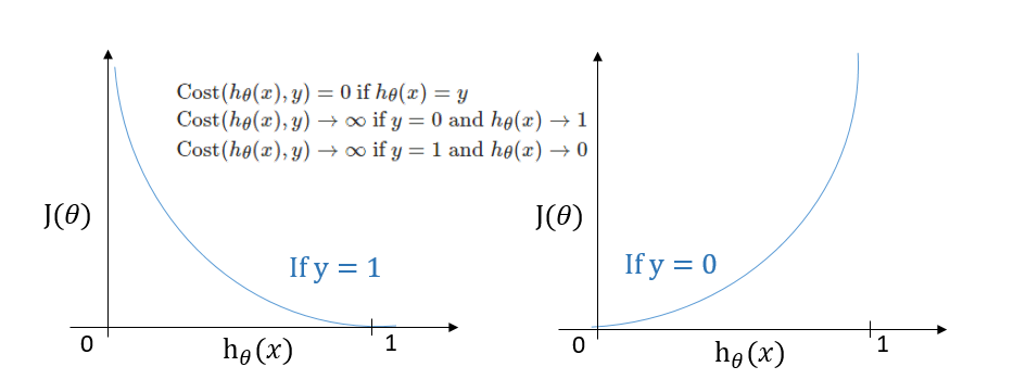
- Compress: $ \displaystyle \mathrm{Cost}(h_\theta(x),y) = -y\log(h_\theta(x)) -(1-y)\log(1-h_\theta(x)) $
- Vectorized implementation:
$ h = g(X\theta) $
$ \displaystyle J(\theta) = \frac{1}{m} \cdot (-y^{T}\log(h)-(1-y)^{T}\log(1-h)) $
Octave: the cost:J = 1/m * (-y' * log(h)-(1-y)'*log(1-h))
the partial derivatives:grad = 1/m * X'*(h-y)
- Gradient Descent
- Repeat {
general form:
$ \displaystyle \theta_j := \theta_j - \alpha \dfrac{\partial}{\partial \theta_j}J(\theta) $
derivative part using calculus:
$ \displaystyle \theta_j := \theta_j - \frac{\alpha}{m} \sum_{i=1}^m (h_\theta(x^{(i)}) - y^{(i)}) x_j^{(i)} $
} - Vectorized implementation:
$\displaystyle \theta := \theta - \frac{\alpha}{m} X^T (g(X\theta) - \vec y) $
- Repeat {
- Optimization algorithm
- Gradient Descent
- Conjugate gradient
- BFGS
- L-BFGS
- Codes in Octave:
function [jVal, gradient] = costFunction(theta)
jVal = [...code to compute J(theta)...];
gradient = [...code to compute derivative of J(theta)...]; end- use octave’s ‘fminunc’ optimization algorithm
options = optimset('GradObj', 'on', 'MaxIter', 100);
initialTheta = zeros(2,1);
[optTheta, functionVal, exitFlag] = fminunc(@costFunction, initialTheta, options);
- use octave’s ‘fminunc’ optimization algorithm
- Multiclass Classification: One-vs-all
- Train a logistic regression classifier for each class i to predict the probability that
$ h_\theta^{(i)}(x) = P(y = i| x;\theta) (i=1,2,\dots,n) $ - On a new input x, to make a prediction, pick the class i that maximizes
prediction = $ \displaystyle\underset{i}{\mathrm{max}} h_\theta^{(i)}(x) $
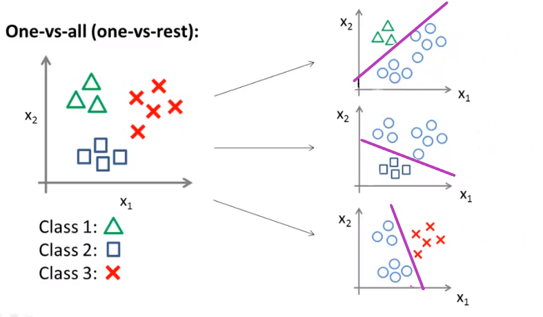
- Train a logistic regression classifier for each class i to predict the probability that
Overfitting
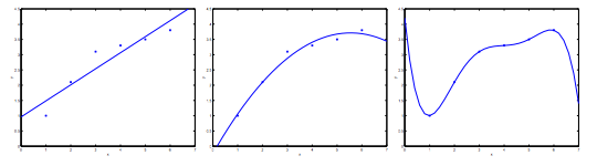
- “Underfit” (“high bias”): not fit the training data very well
- “Just right”
- “Overfit” (“high variance”): may fit the trainning set very well, but fail to generalize to new examples
Regularization
- Using the cost function with the extra summation, we can smooth the output of our hypothesis function to reduce overfitting.
$ min_\theta\, \dfrac{1}{2m}\, \displaystyle[\sum_{i=1}^m (h_\theta(x^{(i)}) - y^{(i)})^2 + \lambda \sum_{j=1}^n \theta_j^2] $ - , or lambda is the regularization parameter
- If lambda is too large, it may cause underfitting.
Linear Regression
-
Gradient Descent:
Repeat {
$ \displaystyle\theta_0 := \theta_0 - \alpha\, \frac{1}{m} \displaystyle\sum_{i=1}^m (h_\theta(x^{(i)}) - y^{(i)})x_0^{(i)} $
$ \displaystyle\theta_j := \theta_j - \alpha\, [ ( \frac{1}{m}\, \sum_{i=1}^m (h_\theta(x^{(i)}) - y^{(i)})x_j^{(i)}) + \frac{\lambda}{m}\theta_j ] $ $ \displaystyle\quad j \in \lbrace 1,2…n\rbrace $
$ \displaystyle\Rrightarrow \theta_j := \theta_j (1- \alpha\,\frac{\lambda}{m}) - \alpha\, \frac{1}{m}\, \sum_{i=1}^m (h_\theta(x^{(i)}) - y^{(i)})x_j^{(i)}) $
} -
Normal Equation:
$ \displaystyle\theta = ( X^TX + \lambda \cdot L )^{-1} X^Ty $
$ \text{where}\, \, L = $
Logistic Regression
- Cost function:
- $ J(\theta) = - \displaystyle\frac{1}{m} \sum_{i=1}^m [ y^{(i)}\, \log (h_\theta (x^{(i)})) + (1 - y^{(i)})\, \log (1 - h_\theta(x^{(i)}))] + \frac{\lambda}{2m}\sum_{j=1}^n \theta_j^2 $
- $ \sum_{j=1}^n \theta_j^2 $ means to explicitly exclude the bias term $ \theta_0 $
- Octave:
- the cost:
J = 1/m * (-y' * log(h)-(1-y)'*log(1-h)) + (lambda/(2*m))*theta'*theta - the partial derivatives:
grad = 1/m * X'*(h-y) + (lambda/m)*theta
- the cost:
- Gradient descent:
- $ \displaystyle h_\theta(x) = \frac{1}{1+e^{-\theta^{T}x}} $
Repeat {
$ \displaystyle\theta_0 := \theta_0 - \alpha\, \frac{1}{m} \displaystyle\sum_{i=1}^m (h_\theta(x^{(i)}) - y^{(i)})x_0^{(i)} $
$ \displaystyle\theta_j := \theta_j (1- \alpha\,\frac{\lambda}{m}) - \alpha\, \frac{1}{m}\, \sum_{i=1}^m (h_\theta(x^{(i)}) - y^{(i)})x_j^{(i)}) $ $ \displaystyle\quad j \in \lbrace 1,2…n\rbrace $
}
- $ \displaystyle h_\theta(x) = \frac{1}{1+e^{-\theta^{T}x}} $
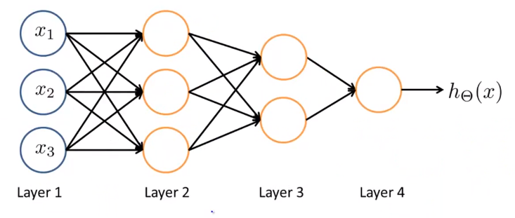
Neural Networks
- Origins: Algorithms that try to mimic the brain
Model representation(NN)
- Neuron model: Logistic unit
- Sigmoid (logistic) activation function: $ g(Z) = \displaystyle\frac{1}{1+e^{-z}} $
- Parameters $ \theta $ also called “weights”
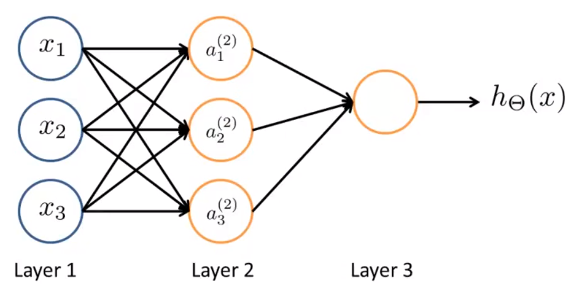
- 1st layer called “input layer”; last layer called “output layer”; middle layers called “hidden layer”
- Notations
- $ x_0 = 1 $ is a “bias unit”
- $ a_i^{(j)} = $ “activation” of unit $ i $ in layer $ j $
- $ \Theta^{(j)} = $ matrix of weights controlling function mapping from layer $ j $ to layer $ j+1 $
- If network has $ s_j $ units in layer $ \displaystyle j, s_{j+1} $ units in layer $ j + 1 $, then $ \Theta^{(j)} $ will be of dimension $ \displaystyle s_{j+1} \times (s_j + 1) $ that
- $ x_0 = 1 $ is a “bias unit”
- Forward propagation: Vectorized implementation
- $ a^{(1)} = x $
- $ \displaystyle z^{(j)} = \Theta^{(j-1)} \ a^{(j-1)} $
- $ \hookrightarrow \displaystyle a^{(j)} = g(z^{(j)} ) $
- Add $ \displaystyle a_0^{(j)} = 1 $
- $ z^{(j+1)} = \Theta^{(j)} a^{(j)} $
- $ \displaystyle h_\Theta(x) = \ a^{(j+1)} = \ g(z^{(j+1)}\ ) $
- Other network architectures
To be continued
-
others: Reinforcement learning, recommender systems
-
Practical advice for applying learning algorithms