This review is for myself further learning to find notations def. & thm. easier
Source of the notes:
Wikipedia
Linear Analysis Lecture Notes
Boundary Value Problems for Linear PDEs
Inverse Problems in Imaging notes

• Common Formul
  • Quick Finding
• Linear Analysis
  • Notations
    • K
    • Delta
    • Class C
    • Multinomial theorem
    • Metric
    • Space
    • Set theoretic Support
    • Test function
    • Inner product
    • Jections
    • Complex
    • Function Space
    • Convolution
    • Null Sequence
  • Theorems and Definitions
    • Morphism
    • Normed Vector Space
    • Vector Space Operation
    • Topological Vector Space
    • Bounded
    • Banach Space
    • Linear Map
    • Operator Norm
    • Dual Space
    • Topologies on Banach Spaces
    • Adjoint Map
    • Finite Dimentional
    • Sublinear
    • Poset
    • Totally Ordered
    • Linearly Independent
    • Extend
    • Hahn Banach
    • Support
    • Dense
    • Baire Category Theorem
    • Interior
    • Meagre
    • Uniform Boundedness
    • Open Mapping Theorem
    • Fubini’s theorem
• Topics in Convex Optimisation
• Bayesian Inverse Problem
• Boundary Value Problems for Linear PDEs
  • Complex Variables
    • Analytic
    • Cauchy Riemann equations
    • Holomorphic
    • dbar Derivative
    • Cauchy’s Theorem
    • Green’s Theorem
    • Residue Theorem
    • Taylor Series
    • Principal Value integrals:
    • Jordan Lemma
    • Fourier Transform
• Inverse Problems in Imaging
  • Notation
  • Introduction
    • Well-Posed
    • Differentiation
    • Fatou lemma
  • Generalised Solutions
    • Orthogonal decomposition
    • Minimal-norm Solutions
    • Decomposition of compact operators
    • Singular Value Decomposition
    • Moore-Penrose inverse
    • Picard criterion
    • ill-posed
  • Regularisation Theory
  • Variational Regularisation
    • Characteristic function
    • Proper
    • Convex
    • Fenchel conjugat
    • Lower-semicontinuous l.s.c
    • Subdifferential
    • Minimiser
    • Weak compact convex subset 4.1.19
    • Bregman distances
    • Absolutely one-homogeneous functionals
    • Coercive
    • Level set
    • J-minimising solutions
    • Main result of well-posedness
    • Total Variation Regularisation
  • Dual Perspective
  • Numerical Optimisation Methods
  • Example
• Topics in Convex Optimisation
• Numerical Solution of Differential Equations
• Calculus
  • Series Expansion

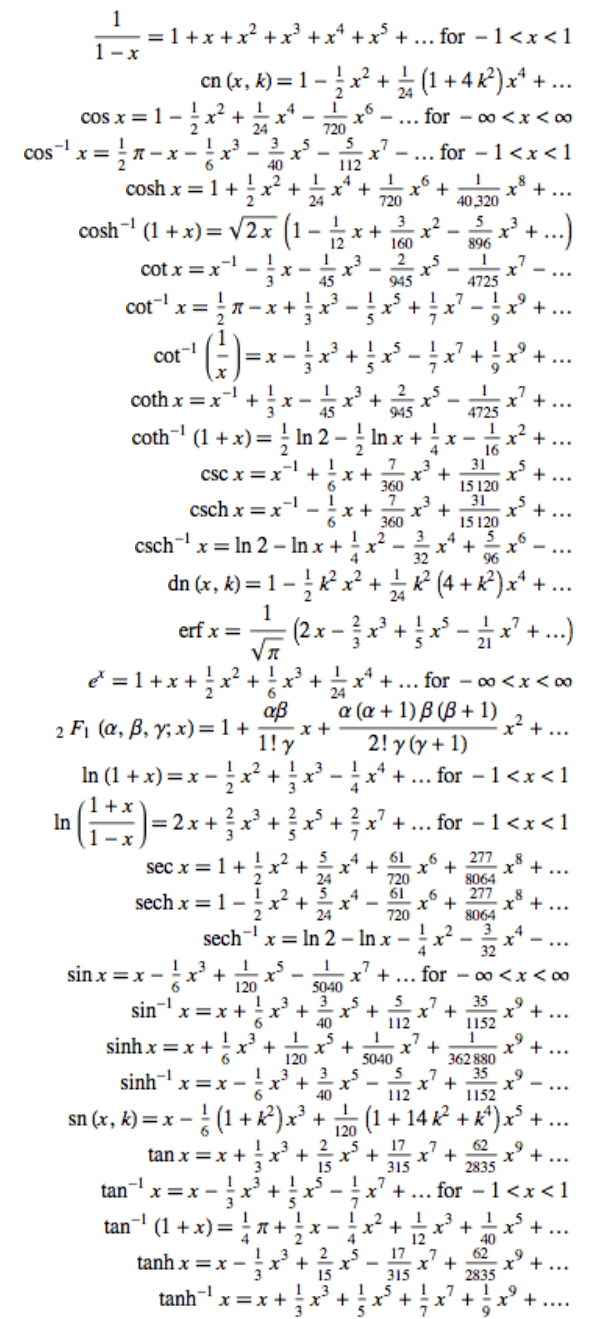
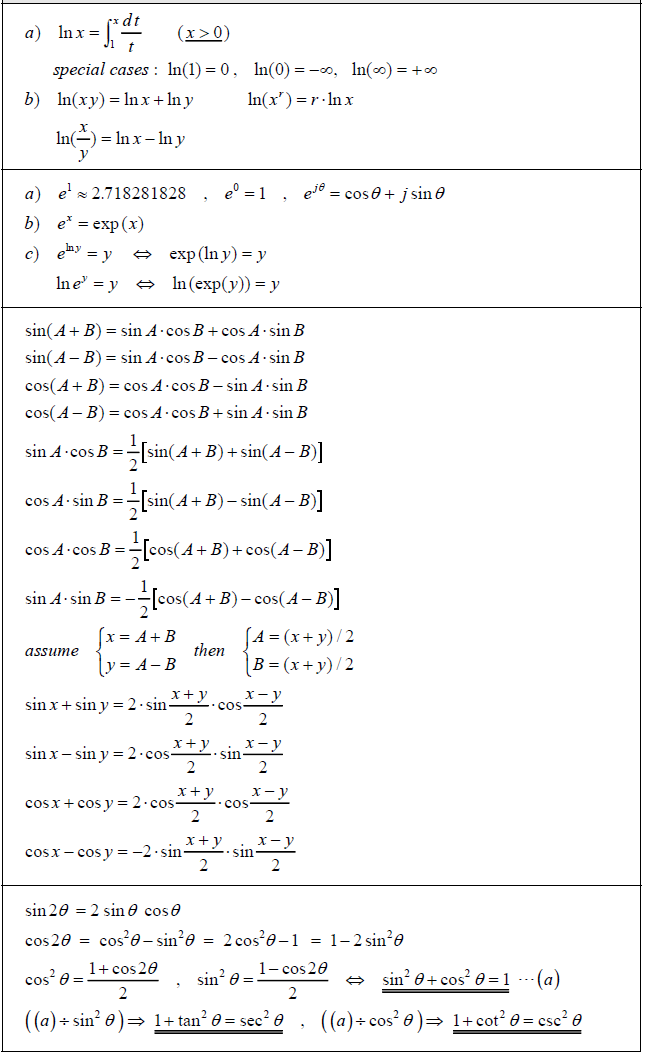
Common Formul

Quick Finding

Fourier Transform
Cauchy’s Theorem
Analytic

f.d.v.s $ \to $ finite dimentional vector space
top. $ \to $ topological
s.t. $ \to $ such that

Linear Analysis

Notations

K

• $ \mathbb{K} $ : real or complex

Delta

• $ \Delta f = \displaystyle \sum_{i=1}^{n} \frac{\partial^2 f}{\partial x_i^2} $
• $ \nabla = (\displaystyle \frac{\partial}{\partial x_1}, \cdots , \frac{\partial}{\partial}) $

Class C

• $ \mathsf{C}^k (Z) $ : the class consists of the complex valued functions on Z which have continuous derivatices of order $ \leq k $
• $ \mathsf{C}^k_c (Z) $ : subset of $ \mathsf{C}^k (Z) $ consisting function with compact support
• $ \mathsf{C}^0_b (Z) $ : the space of all continuous and bounded functions on $ Z $
• $ \mathsf{C}^2_2 (Z) $ : the class of twice continuously differentiable functions that vanish on the exterior of a bounded set
• $ \mathsf{C}^\infty_c (\mathbb{R}^n) $: its members are (complex valued) functions on $ \mathbb{R}^n $ which possess continuous derivatives of all orders and vanish outside some bounded set
  • In distribution theory, it is the basic space of test function
  • also used $ \mathsf{C}^\infty_0 (\mathbb{R}^n) $ and L. Schwartz’s original $ \mathcal{D}(\mathbb{R}^n) $

Multinomial theorem

• Concise form
  • $ (x_1 + \cdots + x_n)^m = \displaystyle \sum_{\lvert \alpha \rvert = m} \frac{m!}{\alpha !} x^\alpha $

Metric

• A metric is defined on V by $ d(v,w) = \lVert v - w \rVert $

Space

• $ \mathfrak{L} (V, W) $ the space of linear maps $ V \to W $
• $ \mathfrak{B} (V, W) $ the space of bounded linear maps $ V \to W $
• $ \mathfrak{K} (V, W) $ the space of compact operators

Set theoretic Support

• The set-theoretic support of $ f ： X \to \mathbb{R} $ where X arbitrary set, written supp(f), is the set of points in X where f is non-zero
  $ supp(f) = { x \in X \mid f(x) \neq 0 } $
  • If $ f(x) = 0 $ for all but a finite number of points x in X, then f is said to have finite support

Test function

• $ C^\infty_0 $ test functions are the test function with the following properties
  • infinitely differentiable
  • compact [Support]
• All of it derivatives will vanish smoothly

Inner product

• Inner product: $ f_v(w) $ $ = < w, v > $

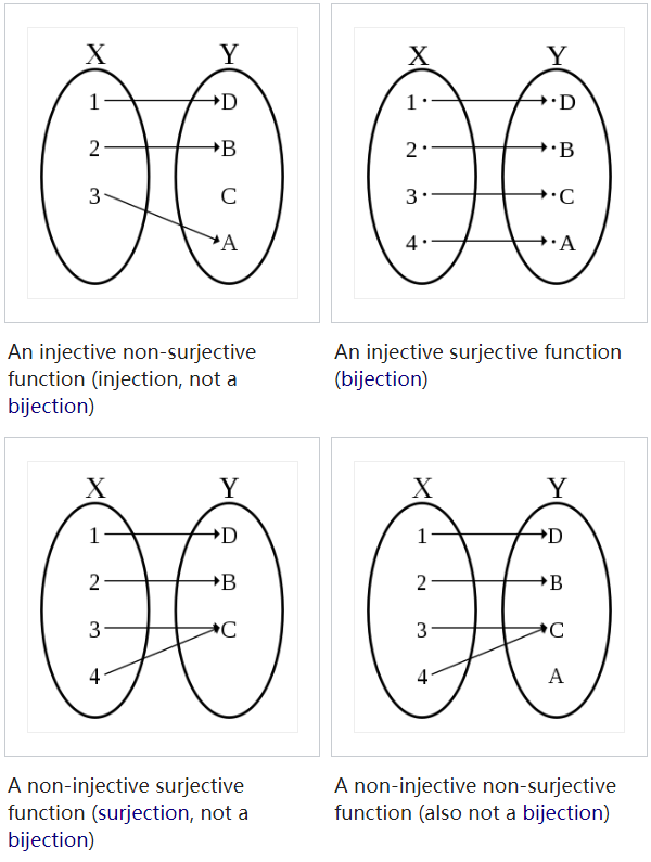
Jections

• Injections $ \hookrightarrow $
• Surjections $ \twoheadrightarrow $
• Bijections $ \xrightarrow{\sim} $
  

Complex

• $ \lvert z \rvert = \sqrt{x^2 + y^2} = \rho $ the length of the complex number z
• $ x = \rho \cos \theta , \; y = \rho \sin \theta $
  $ z = \rho (\cos \theta + i \sin \theta) $
• Crucial identity
  $ e^{i\theta}= \cos \theta + i \sin \theta $
  $ z = \rho e^{i\theta} ,\; \rho > 0 ,\; \theta $ real
  $ e^{i\theta + 2i\pi m} = e^{i\theta},\; m \in \mathbb{Z}$

Function Space

• $ C^0 (U) = \lbrace u: U \to \mathbb{R} \mid u $ continuous }
• $ C (\bar{U}) = \lbrace u: \in C(U) \mid u $ uniformly continuous }
• $ C^k (U) = \lbrace u: U \to \mathbb{R} \mid u $ is k-times continuously differentiable }
  • $ C^\infty (U) = \cap_{k=0}^{\infty} C^k (U) = C^\infty (\bar{U}) = \cap_{k=0}^{\infty} C^\infty (\bar{U}) $
• $ L_p \mathrm{or} L^p $ function space
  • $ L_p (U) = \lbrace u : U \to \mathbb{R} \mid \lvert u \rvert_{L^p(U)} < \infty \rbrace $ where u is Lebesgue measurable
    • $ \lVert u \rVert_{L^p(U)} = \displaystyle (\int_{U} \lvert f \rvert^p dx )^{\frac{1}{p}}, (1< p < \infty) $

Convolution

• If $ f, g : \mathbb{R}^n \to \mathbb{C} $, then the convolution is :
  • $ (f \star g)(x) = \displaystyle \int_{\mathbb{R}^n} f(y) g(x-y) dy $
• If $ f, g, h \in C_0^\infty (\mathbb{R}^n) $
  • $ f \star g = g \star f $
  • $ f \star (g \star h) = (f \star g) \star h $
  • $ \displaystyle \int_{\mathbb{R}^n} (f \star g)(x) dx = \displaystyle \int_{\mathbb{R}^n} f (x) dx \displaystyle \int_{\mathbb{R}^n} g (x) dx $
• Support $ f \in L_{loc.}^1 (\mathbb{R}^n), g \in C_0^k (\mathbb{R}^n) $ for some $ k \geq 0 $, then $ (f \star g) \in C^k(\mathbb{R^n}) $ and
  • $ D^\alpha(f \star g) = f \star D^\alpha g , \lvert \alpha \rvert \leq k $

Null Sequence

• Null sequence $ \lbrace \sigma_j \rbrace_{j \in \mathbb{N}} $ is a sequence converges to a limit of 0:
  • $ \displaystyle \lim_{j \to \infty} \sigma_j = 0 $

Theorems and Definitions

Morphism

• A category $ \mathsf{C} $ consists of
  • a class $ Obj(\mathsf{C}) $ of objects of the category
  • for every two objects $ A $, $ B $ of $ \mathsf{C} $, a set $ Hom_\mathsf{C} (A, B) $ of morphisms, with the properties below:
    1. For every object $ A $ of $ \mathsf{C} $,
       $ \exists I_A \in Hom_\mathsf{C} (A, A) $ the identity of $ A $
    2. One can compose morphism:
       Two morphisms $ f \in Hom_\mathsf{C}(A, B) $ and $ g \in Hom_\mathsf{C}(B, C) $ determine a morphism $ gf \in Hom_\mathsf{C}(A, C) $
       There is a function (of sets)
       $ Hom_\mathsf{C}(A, B) \times Hom_\mathsf{C}(B, C) \to Hom_\mathsf{C}(A, C) $
       and the image of the pair $ (f, g) $ is denoted $ g f $
    3. Associative: $ h \in Hom_\mathsf{C}(C, D) $
       $ (hg)f = h(gf) $
    4. Identity morphisms are identities
       $ f I_A = f, \; \; I_B f = f $
    5. the sets $ Hom_\mathsf{C} (A, B), \; Hom_\mathsf{C} (C, D) $ be disjoint unless $ A = C, B = D $

• Homomorphism
  A homomorphism is a map between two algebraic structures of the same type, that preserves the operations of the structures
  Formally, a map $ {\displaystyle f:A\to B} $ preserves an operation $ \mu $ of arity $ k $, defined on both $ A $ and $ B $ if
  $\displaystyle f(\mu_{A}(a_{1},\ldots ,a_{k}))=\mu_{B}(f(a_{1}),\ldots ,f(a_{k})), $
  for all elements $ a_1, …, a_k \in A $

• Endomorphism
  A morphism od an object $ A $ of a category $ \mathsf{C} $ to itself
  $ Hom_\mathsf{C}(A, A) $ is denoted $ End_\mathsf{C} (A) $

• Mono-morphism (or Monic)
  • A function $ f : A \to B $ is a mono-morphism (or monic) if holds:
    for all sets $ Z $ and all functions $ \alpha^\prime, \alpha^{\prime\prime} : Z \to A $
    (for all objects $ Z $ of $ \mathsf{C} $ and all morphisms $ \alpha^\prime, \alpha^{\prime\prime} \in Hom_\mathsf{C}(Z, A) $ )
    $ f \circ \alpha^\prime = f \circ \alpha^{\prime\prime} \to \alpha^\prime = \alpha^{\prime\prime} $
  • A function is injective iff it is a monomorphism
• Epimorphism
  • for all objects $ Z $ of $ \mathsf{C} $ and all morphisms $ \beta^\prime, \beta^{\prime\prime} \in Hom_\mathsf{C}(B, Z) $
    $ \beta^\prime \circ f = \beta^{\prime\prime} \circ f \to \beta^\prime = \beta^{\prime\prime} $
  • A function is surjective iff it is epimorphism
• Isomorphism
  • A morphism $ f \in Hom_\mathsf{C} (A, B) $ is isomorphism if it has a (two sided) inverse under composition: that is
    if $ \exists g \in Hom_\mathsf{C}(B, A) $ s.t. $ gf = I_A, fg = I_B $
  • The inverse of an isomorphism is unique
  • prop.
    • Each identity $ I_A $ is an isomorphism and is its own inverse
    • If $ f $ is an isomorphism, then $ f^{-1} $ is also and $ (f^{-1})^{-1} = f $
      If $ f, g $ are isomorphisms, the $ gf $ is also and $ (gf)^{-1} = f^{-1}g^{-1} $

• Endomorphism
  An endomorphism is a homomorphism whose domain = codomain, or
  A morphism whose source is equal to the target
  

• Automorphism
  An automorphism is an endomorphism also an isomorphism

Normed Vector Space

• Normed Vector Space is a vector space (v.s.) V with a norm $ \lVert \cdot \rVert \ : \ V \to \mathbb{R}, \ v \mapsto \lVert v \rVert $ satisfying:
  1. $ \lVert v \rVert \geqslant \ \forall \ v \in V \ \mathrm{and} \ \lVert v \rVert = 0 \ \mathrm{iff} \ v = 0 $ (pos. def)
  2. $ \lVert \lambda v \rVert = \lvert \lambda \rvert \lVert v \rVert $ for every $ \lambda \in \mathbb{k} $ and $ v \in V $ (pos. homogeneity)
  3. $ \lVert v \ + \ w \rVert \ \leqslant \ \lVert v \rVert + \lVert w \rVert $ for every $ v, w \in V $ (triangle ineq.)
• If $ V $ is a separable normed space, then $ V $ embeds isometrically into $ l_\infty $

Vector Space Operation

• Vector Space Operations are continuous maps
  • $ \mathbb{K} \times V \to V , (\lambda , v) \mapsto \lambda v $ (scalar multi.)
  • $ V \times V \to V , (v , w) \mapsto v + w $ (addition)

Topological Vector Space

• Topological Vector Space (top.) is a vector space together with a topology which makes the vector space operations continuous and points are closed

Bounded

• Let V be a topological vector space and $ B \subset V $
  We say that B is bounded if
  for every open neighbourhood u of 0, there exists $ t > 0 $
  s.t. $ sU \supset B \; \forall \; s \geq t $

Banach Space

• a Banach Space is a normed vector space that is complete as a metric space
  i.e. every Cauchy sequence converges
• Let V be a normed space and W a Banach space. Then $ \mathfrak{B} (V, W) $ is a Banach space
• Let V be a normed v.s. then $ V^{\star} $ is a Banach space
• Vector-valued Liouville’s Theorem
  Let X be a comple Banach Space, and $ f: \mathbb{C} \to X $ a bounded analytic function
  then $ f $ is constant

Linear Map

• In any topological vector spaces V, W ;
  a linear map $ T: V \to W $ is countinuous iff it is countinuous at 0

• T is bounded if $ T(B) $ is bounded for any bounded $ B \subset V $

Fact.

• If V,W are normed v.s., a linear map $ T : V \to W $ is bounded iff
  there is a $ \lambda > 0 $ s.t. $ T (B_1(0)) \subseteq B_\lambda (0) $
  i.e. $ \lVert TV \rVert \leq \lambda \; \forall \; v \in V $ with $ \lVert v \rVert \leq 1 $

Operator Norm

• Let V,W be normed v.s.
  The operator norm of a linear map $ T : V \to W $ is
  $\displaystyle \lVert T \rVert = \sup_{\lVert v \rVert = 1} \lVert Tv \rVert = \sup_{\lVert v \rVert \leq 1} \lVert Tv \rVert = \sup_{\lVert v \rVert < 1} \lVert Tv \rVert$
• Denote by $ \mathfrak{L} (V, W) $ the space of linear maps $ V \to W $
  by $ \mathfrak{B} (V, W) $ the space of bounded linear maps $ V \to W $

Fact.

• The operator norm $ \lVert \cdot \rVert $ is a norm on $ \mathfrak{B} (V, W) $

Prop.

• Let V,W be normed v.s.
  Then a linear map $ T : V \to W $ is bounded iff it is countinous

Dual Space

• Let V be a top. v.s.
  The $ V^{\star} $ (top.) dual space of V is the space of all continuous linear maps $ V \to \mathbb{K} $
  • We call $ \mathfrak{L} (V, \mathbb{k}) $ the algebraic dual of V

• Let V be a normed v.s.
  The double dual of V is the dual space of $ V^{\star} $
  i.e. $ V^{\star \star} = (V^{\star})^{\star} $
  $ V^{\star\star} $ is also called bidual or the second dual of $ V $
  For each $ x \in X $, define $ \hat{x} : X^\star \to $ scalars by $ \hat{x}(f) = f(x) $
  then $ \hat{x} $ is linear, and $ \lvert \hat{x} (f) \rvert = \lvert f(x) \rvert \leq \lVert f \rVert \cdot \lVert x \rVert $
  so $ \hat{x} \in X^{\star\star} $ with $ \lVert \hat{x} \rVert \leq \Vert f \rVert $

• If X be a normed space
  The dual space $ X^\star $ is the space of all bounded linear functionals on $ X $
  This is a normed space with norm $ \lVert f \rVert = \sup{\lvert f(x) \rvert : x \in B_X } $ , where $ B_X = { x \in X : \lVert x \rVert \leq 1} $
  $ X^\star $ is always complete

Fact.

• The map $ \phi : V \to V^{\star \star} $ , $ v \mapsto \tilde{v} $ where $ \tilde{v} (f) = f(v) $ is bounded and linear

• A Banach space is reflexive if $ \phi $ is bijection

• Dual operators

  Define the dual operator of $ T $ by $ T^\star : X^\star \to Y^\star , T^\star (g) = g \circ T $ for $ g \in Y^\star $
  This is well-defined as $ g \circ T $ is a composition of bounded linear operators
  Furthermore, $ T^\star $ is linear and bounded, since
  $\begin{align*} \lVert T^\star \rVert & = \sup_{g \in B_{Y^\star}} \lVert T^\star g \rVert = \sup_{g \in B_{Y^\star}} \sup_{x \in B_{X}} \lvert \langle x, T^\star y \rangle \rvert \\ & =\sup_{x \in B_{X}} \sup_{g \in B_{Y^\star}} \lvert \langle T^\star y \rangle \rvert = \sup_{x \in B_X} \lVert T x \rVert = \lVert T \rVert \end{align*}$

Topologies on Banach Spaces

• Let $ (X, \lvert . \rvert) $ denote a real Banach space
• $ \displaystyle X^\star = { l : X \to R \ \mathrm{linear \ s.t. } \lvert l \rvert_{X^\star} = \sup_{x\neq 0} \frac{\lvert l(x) \rvert}{\lvert x \rvert_X} \leq \infty } $
• Topologies on $ X $
  1. The strong topology $ x_n \displaystyle \longrightarrow_{X} x $ defined by
     $ \lvert x_n - x \rvert_X \to 0 \ (n \to +\infty) $
  2. The weak topology $ x_n \displaystyle \longrightarrow_{X} x $ defined by
     $ l(x_n) \to l(x) \ (n \to +\infty) $ for every $ l \in X^\star $
• Topologies on $ X^\star $
  1. The strong topology $ l_n \displaystyle \longrightarrow_{X} l $ defined by
     $ \lvert l_n - l \rvert_{X^\star} \to 0 \ (n \to +\infty) $
     or equivalently,
     $ \sup_{x\neq 0} \frac{\lvert l_n(x) - l(x) \rvert}{\lvert x \rvert_X} \to 0 \ (n \to +\infty) $
  2. The weak topology $ x_n \displaystyle \longrightarrow_{X} x $ defined by $ l(x_n) \to l(x) \ (n \to +\infty) $ for every $ l \in X^\star $

Adjoint Map

• Let V,W be normed v.s. and $ T \in \mathfrak{B}(V, W) $
  Then the adjoint map $ T^{\star} : W^{\star} \to V^{\star} $ is defined by
  $ [T^{\star} f] v = f (T v) \; \mathrm{for} \; f \in W^{\star}, v \in V $

Fact.

• $ T^\star f $ is indeed in $ V^\star = \mathfrak{B} (V, \mathbb{K}) $ and $ \lVert T^\star \rVert \leq \lVert T \rVert $

Finite Dimentional

• Any finite-dimensional vector space can be identified with $ \mathbb{K}^n $ by choosing a basis. there n is the dimension
• Two norms $ \lVert \cdot \rVert $ and $ \lvert \lVert \cdot \rVert \rvert $ on a vector space V are equivalent iff
  there exists a constant $ C > 0 $ s.t.
  $ C^{-1} \lvert \lVert v \rVert \rvert \leq \lVert v \rVert \leq C \lvert \lVert v \rVert \rvert $ for all $ v \in V $

Prop.

• All norms on a f.d.v.s. are equivalent
• In any f.d.v.s., the closed unit ball is compact
• Every f.d. normed v.s. is a Banach space
• Let V be a normed v.s. and $ W \subset V $ be a f.d. subspace, then W is closed

Thm.

• Let V be a normed v.s. s.t. $ \overline{B_1(0)} $ is compact. Then V is finite-dimentional

Sublinear

• a map $ p : V \to \mathbb{R} $ is sublinear if
  1. $ p( \alpha v ) \ = \ \alpha \ p(v) \; \forall v \in V , \ \alpha \geq 0 $
  2. $ p(v+w) \ \leq \ p(v) + p(v) \; \forall v,\ w \in V $

Poset

• A partially ordered set (poset) is a set P with a binary relation $ \leq $ s.t. for all $ x, y \in P $ either $ x \leq y $ or $ x \nleq y $ , and
  $ x \leq x $ (reflexive)
  $ x \leq y , y \leq z \; \Rightarrow \; x \leq z $ (transitive)
  $ x \leq y , y \leq x \; \Rightarrow \; x = y $ (antisymmetric)

• Let P be a poset. An element $ m \in P $ is maximal if $ m \leq x \to m = x $

Totally Ordered

• Let P be a poset. a subset $ T \subset P $ is called totally ordered (or a chain) if
  $ x \nleq y \Rightarrow y \leq x $
  i.e.
  either $ x \leq y or y \leq x $

Linearly Independent

• In a v.s. V, elements $ v_1, \cdots , v_k $ are linearly independent if
  $ \sum_{i = 1}^{k} \alpha_i v_i = 0 \; \to \; \alpha_1 = \alpha_2 = \cdots = 0 $
• a set $ S \subset V $ is linearly independent if any finite subset is
• A basis of V is a set $ B \subset V $ that is linearly independent and such that every element of V is a finite linear combination of elements in B

Prop.

• Let $ V \neq \lbrace 0 \rbrace $ be a vector space and $ S \subset V $ linearly independent. Then V has a basis B s.t. $ S \subset B $

Extend

• Given vector spaces $ W \subset V $ , linear maps $ g : W \to \mathbb{K} , f : V \to \mathbb{K} $ , we say that f extends g if $ f \lvert_{w} = g $

Hahn Banach

• Let V be a real vector space, a subspace $ W \subset V , p : V \to \mathbb{R} \; \mathrm{sublinear}, g: W \to \mathbb{R} $ linear s.t.
  $g(v) \leq p(v) \; \forall v \in W$
  Then there is $ f : V \to \mathbb{R} $ linear s.t. $ f\lvert_W = g $ and
  $f(v) \leq p(v) \; \forall v \in V$

Cor.

• Let $ V \in \mathbb{K} $ be a normed v.s., $ W \subset V $ a subspace
  For any $ g \in W^\star $ there exists $ f\in V^{star} $
  s.t. $ f\lvert_{W} = g $ and $ \lVert f \rVert \leq \lVert g \rVert $
• Let V be a normed vector space and $ v \in V $
  Then $ \exists f_v \in V^\star $ s.t. $ \lVert f_v \rVert = 1 $ and $ f_v (V) = \lVert v \rVert $
  • Here $ f_v $ is called a support functional for V
• Let V be a normed v.s. and $ v \in V $ , then
  $ v = 0 \Leftrightarrow f(v) = 0 \; \forall \; f \in V^\star $
  In particular, $ V^\star \neq 0 $
• Let V be a normed v.s., $ v, w \in V , \ v \neq w $ . Then
  there exists $ f \in V^\star $ s.t. $ f(v) \neq f(w) $

Prop.

• The map $ \phi : V \to V^{\star \star } $ is an isometry
  ($ d_Y(f(x),f(y)) = d_X(x,y) $ for a map $ f: X \to Y $) that
  $ \lVert \phi (v) \rVert = \lVert v \rVert $
• Let V, W be a normed v.s.
  For any $ T \in \mathfrak{B} (V, W) $ , the dual map $ T^\star \in \mathfrak{B} (W^\star, V^\star ) $ satisifies $ \lVert T^\star \rVert = \lVert T \rVert $

Support

• If the domain of f is a top. space, the support of f is the smallest closed set containing all points not mapped to zero

Closed Support:

• The support of f is defined topologically as the closure of the subset of X where f is non-zero
• support of a function $ f : X \to \mathbb{C} $ is the closure of the set $ \lbrace x \in X \mid f(x) \neq 0 \rbrace $; it is the closed subset of X
  i.e. $ supp(f) := \overline{\lbrace x \in X \mid f(x) \neq 0 \rbrace} $ $ = \overline{f^{-1}(\lbrace 0 \rbrace^c)} $

Compact Support:

• The closed support is a compact subset of $ X $
• If $ X $ is the real line, or n-dimensional Euclidean space, then a function has compact support iff it has bounded support
• Each function is nonzero on a closed and bounded interval, but is zero everywhere else

Essential Support:

• If X is a top. measure space with a Borel measure μ
  the essential support of a measurable function $ f : X \to \mathbb{R} $, written ess supp(f), is defined to be the smallest closed subset $ F $ of $ X $ such that $ f = 0 $ μ-almost everywhere outside $ F $
  Equivalently, ess supp(f) is the complement of the largest open set on which f = 0 μ-almost everywhere $ \displaystyle \mathrm{ess supp}(f) := X \setminus \bigcup \lbrace \Omega \subset X \mid \Omega $ is open and $ f = 0 $ μ-almost everywhere in $ \Omega \rbrace $

Support Function:

• The support function $ h_A : \mathbb{R}^n \to \mathbb{R} $ of a non-empty closed convex set A in $ \mathbb{R}^n $ is given by
  $ h_A (x) = sup \lbrace x \cdot a : a \in A \rbrace , \; x \in \mathbb{R}^n $

Supporting Functional:
In convex analysis and mathematical optimization, the supporting functional is a generalization of the supporting hyperplane of a set

• Let X be a locally convex top. space and $ C \subset X $ be a convex set, then
  the continuous linear functional $ \phi : X \to \mathbb{R} $ is a supporting functional of C at the point $ x_0 $
  if $ \phi(x) \leq \phi(x_0) $ for every $ x \in C $
• If $ h_C : X^\star \to \mathbb{R} $ is a support function of the set C, then
  if $ h_C (x^\star) = x^\star (x_0) $ , it follows that
  $ h_C $ defines a supporting functional $ \phi : X \to \mathbb{R} $ of $ C $ at the point $ x_0 $ s.t.
  $ \phi(x) = x^\star (x) $ for any $ x \in X $
• If $ \phi $ is a supporting functional of the convex set C at the point $ x_{0} \in C $ such that
  $ \displaystyle \phi (x_{0}) = \sigma = \sup_{x \in C} \phi (x) > \inf_{x \in C} \phi (x) $
  then $ H = \phi^{-1} (\sigma ) $ defines a supporting hyperplane to C at $ x_{0} $

Dense

• If X is a metric space, the $ Y \subset X $ is dense if $ \overline{Y} = X $
  i.e. $ Y \cap B_r (X) \neq \varnothing \; \forall \; x \in X , r > 0 $

Baire Category Theorem

• Let X be a complete metric space.
  For any sequence of open dense subsets $ U_j \subset X $ , $ \displaystyle\bigcap_j U_j $ is dense in $ X $

cor.

• Let $ X $ be a complete metric space. Let $ A_j \subset X $ be a sequence of closed subsets s.t.
  $ \bigcup_j A_j $ has nonempty interior, i.e. it contains some ball
  Then at least one of the $ A_j $ has nonempty interior

Interior

• The point x is an interior point of S. The point y is on the boundary of S
  
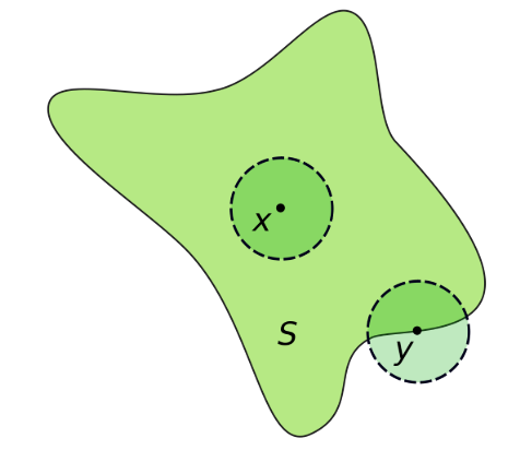
• Interior point
  If $ S $ is a subset of a Euclidean space, then $ x $ is an interior point of $ S $ if there exists an open ball centered at $ x $ which is completely contained in S
• Interior of a set
  The interior of a set $ S $ is the set of all interior points of $ S $
  it is denoted $ int(S) $, $ Int(S) $ or $ S^o $
  and has the following properties:
  • $ int(S) $ is an open subset of $ S $
  • $ int(S) $ is the union of all open sets contained in $ S $
  • $ int(S) $ is the largest open set contained in $ S $
  • A set $ S $ is open iff $ S = int(S) $
  • $ int(int(S)) = int(S) $ (idempotence)
  • If $ S $ is a subset of $ T $, then $ int(S) $ is a subset of $ int(T) $
  • If $ A $ is an open set, then $ A $ is a subset of $ S $ iff $ A $ is a subset of $ int(S) $

Meagre

• Let X be a metric space
  1. A subset $ Y \subset X $ is nowhere dense if $ int( \overline{Y} ) = \varnothing $ ,
     ( if the interior of its closure is empty )
     i.e. , if $ Y $ is not dense in any ball
  2. A subset $ Z \subset X $ is meagre or of the first category if
     there are countably many set $ Y_j \subset X $ that are nowhere dense and $ Z = \bigcup_j Y_j $
     ( if it is a union of countably many nowhere dense subsets )
  3. A subset $ U \subset X $ is nonmeagre or of the second category if it is not meagre
     ( it contains a countable union of open and dense sets )
  4. A subset $ R \subset X $ is residual if
     its complement is meagre

fact.

• $ Y \subset X $ is nowhere dense
  $ \Leftrightarrow \; \overline{Y} $ is nowhere dense
  $ \Leftrightarrow \; X \backslash \overline{Y} $ is open dense

Cor.

• Let $ X $ be a complete metric space. Then $ X $ is of second category
• Let $ X $ be a complete metric space. Then residual sets are non-meagre and dense
• Let $ X $ be a complete metric space and $ U \subset X $ open.
  Then $ U = \varnothing $ or $ U $ is of the second category

Uniform Boundedness

• Principle of uniform boundedness
  Let X be a complete metric space
  Let $ (f_\lambda)\mid_{\lambda \in \wedge} $ be a family of continuous functions $ f_\lambda : X \to \mathbb{R} $
  If $ (f_\lambda)\mid_{\lambda \in \wedge} $ is pointwise bounded,
  i.e., $ \sup_{\lambda \in \wedge} \lvert f_\lambda (x) \rvert \leq \infty $ for every $ x \in X $,
  then there is a ball $ B_r (X_c) \subset X $ s.t.
  $ ( f_\lambda ) $ is uniformly bounded on $ B_r(X_0) $
  i.e., $ \sup_{\lambda \in \wedge} \sup_{x \in B_r (x_0)} \lvert f_\lambda (x) \rvert \leq \infty $

• Banach-Steinhaus Theorem
  Let $ V $ be a Banach Space and $ W $ a normed v.s.
  Let $ (T_\lambda)\mid_{\lambda \in \wedge} \subset \mathfrak{B}(V,W) $ be pointwise bounded,
  i.e., $ \sup_{\lambda \in \wedge} \lVert T_\lambda v \rVert \; \forall \; v \in V $
  Then $ ( T_\lambda) $ is uniformly bounded
  i.e., $ \sup_{\lambda \in \wedge} \lVert T_\lambda \rVert \leq \infty $

Open Mapping Theorem

• A map between topological spaces is open iff it maps open ses to open sets

• Open Mapping Theorem
  Let $ V, W $ be Banach Spaces and $ T \in \mathfrak{B} (V, W) $

  1. if $ T $ is surjective, then $ T $ is open
  2. if $ T $ is bijective, then $ T^{-1} \in \mathfrak{B}(W, V) $

Fubini’s theorem

• If $ f(x,y) $ is $ X \times Y $ integrable, that $ f(x,y) $ is measrable function and $ \displaystyle \int_{X \times Y} \lvert f(x,y) \rvert d(x,y) < \infty $ then
  • $ \displaystyle \int_{X} (\int_{Y} f(x,y)dy)dx = \int_{Y}(\int_{X} f(x,y) dx) dy = \int_{X \times Y}f(x,y) d(x,y) $

Topics in Convex Optimisation

Bayesian Inverse Problem

Boundary Value Problems for Linear PDEs

Complex Variables

Analytic

• $ f(z) = u(x, y) + iv(x, y) $ where $ u , v $ are real functions
  We called $ f(z) $ an analytic at point $ z_0 $
  if it is differentiable in a neighbourhood of $ z_0 $
• $ f(z) $ is analytic iff functions $ u , v $ satisfy Cauchy–Riemann equations

• $ f $ is an analytic function iff dbar-Derivative
  $\displaystyle \frac{\partial f}{\partial \bar{z}} = 0 $ or $ \displaystyle \frac{\partial f}{\partial z} = u_x - i u_y = v_y + i v_x $

• Liouville’s theorem:
  If $ f(z) $ is everywhere analytic (in the finite complex plane) and bounded (including infinity), then $ f(z) $ is a constant.

• Rouche’s theorem:
  Let $ f(z) $ and $ g(z) $ be analytic on and inside a simple contour $ C $.
  If $ |f(z)| > |g(z)| $ on $ C $, then $ f(z) $ and $ f(z) + g(z) $ have the same number of zeros inside the contour $ C $.

• Morera’s theorem:
  If $ f(z) $ is continuous in a domain $ D $ and if
  $ \displaystyle \oint_C f(z) dz = 0 $
  for every simple closed contour $ C $ lying in $ D $,
  then $ f(z) $ is analytic in $ D $.

• Maximum Principle:
  If $ f(z) $ is analytic in a bounded region $ D $
  and $ \lvert f(z) \rvert $ is continuous in the closed region $ \bar{D} $,
  then $ \lvert f(z)\rvert $ obtains its maximum on the boundary of the region

• Minimum Principle:
  If, in addition, it is non-zero at all points of $ D $, then $ \lvert f(z) \rvert $ obtains its minimum on the boundary of the region.

• Laurent Series:
  A function $ f(z) $ analytic in an annulus(环) $ R_1 < \lvert z - z_0 \rvert < R_2 $ may be presented by the expansion
  $ f(z) = \displaystyle\sum_{m=-\infty}^{\infty} A_m(z-z_0)^m $
  where $ A_m = \displaystyle \frac{1}{2i\pi} \oint_C \frac{f(z)dz}{(z-z_0)^{m+1}} $
  and $ C $ is any simple closed contour in the region of analyticity enclosing the inner boundary $ \lvert z - z_0 \rvert = R_1 $.

Cauchy Riemann equations

• The Cauchy–Riemann equations on a pair of real-valued functions of two real variables $ u(x,y) $ and $ v(x,y) $ are the two equations:
  1. $ \displaystyle \frac{\partial u}{\partial x} = \frac{\partial v}{\partial y} $
  2. $ \displaystyle \frac{\partial u}{\partial y} = - \frac{\partial v}{\partial x} $
     That $ u_x = v_y , \; u_y = - v_x $

Holomorphic

• Holomorphy is the property of a complex function of being differentiable at every point of an open and connected subset of $ C $ (a domain in $ C $)
• If f is complex-differentiable at every point $ z_0 $ in an open set $ U $, we say that $ f $ is holomorphic on $ U $.
  We say that $ f $ is holomorphic at the point $ z_0 $ if it is holomorphic on some neighbourhood of $ z_0 $.
• In complex analysis, a function that is complex-differentiable in a whole domain (holomorphic) is the same as an analytic function
  NOT true for real differentiable functions
• Any holomorphic function is actually infinitely differentiable and equal to its own Taylor series (analytic)

dbar Derivative

• the dbar-derivative with respect to $ \bar{z} $
  i.e. the derivative with respect to the complex conjugate of $ z $
  The equations $ z = x + iy , \; \bar{z} = x - iy $
  imply $ x = \displaystyle \frac{z+\bar{z}}{2} , \; y = \frac{z-\bar{z}}{2i} $
  Chain rule yields
  $ \displaystyle \frac{\partial}{\partial z} = \frac{1}{2} (\frac{\partial}{\partial x}-i\frac{\partial}{\partial y}) , \; \displaystyle \frac{\partial}{\partial \bar{z}} = \frac{1}{2} (\frac{\partial}{\partial x}+i\frac{\partial}{\partial y}) $

Cauchy’s Theorem

Cauchy integral theorem (also known as the Cauchy–Goursat theorem)

• Suppose that $ f(z) $ is analytic in the domain $ D $.
  Then, the integral of $ f(z) $ along the boundary of $ D $ vanishes.

Green’s Theorem

• Let $ C $ be a positively oriented, piecewise smooth, simple closed curve in a plane, and let $ D $ be the region bounded by $ C $.
  If $ L $ and $ M $ are functions of $ (x, y) $ defined on an open region containing $ D $ and have continuous partial derivatives there, then
  $ \displaystyle \oint_C (L dx + M dy) = \int \int_D (\frac{\partial M}{\partial x} - \frac{\partial L}{\partial y}) dx dy $
  where the path of integration along C is anticlockwise

Residue Theorem

• Suppose that the function $ f(z) $ is analytic in the domain $ D $,
  except at the single point $ z_0 $ where the function has a pole with residue $ g(z_0) $, namely in the neighborhood of $ z_0 $, this function can be written as
  $ f(z) = \displaystyle \frac{g(z)}{z - z_0} $ where $ g(z) $ is analytic.
  Then, the integral of $ f(z) $ along the boundary of $ D $ equals $ 2i\pi g(z_0) $

• Cauchy’s Residue Theorem

• $ \oint_C f(z)dz = 2 \pi i \displaystyle \sum_{k = 1}^n \mathrm{Res} (f(z), z_k) $
• If $ z_k $ is a pole of order k, then the residue of f around $ z = z_k $ can be found by the formula:
  Res $ (f , z_k) = \displaystyle \frac{1}{(k-1)!} \lim_{z\to z_k} \frac{d^{k-1}}{dz^{k-1}} ((z-z_k)^k f(z)) $
• For essential singularity case, the residues must usually be taken directly from series expansions

Taylor Series

• Analytic real function can be expanded in terms of an infinite series:
  $f(x) = \displaystyle \sum_{m=0}^\infty \frac{(x-x_0)^m}{m!} \frac{d^m}{dx^m} f(x_0)$
  where this series is valid provided that $ \lvert x - x_0 \rvert < R $ and $ R $ is called the radius of convergence

• Complexification
  Let $ f(z) $ be analytic for $ \lvert z - z_0 \rvert < R $
  Then $ f(z) = \displaystyle \sum_{m=0}^\infty \frac{(z-z_0)^m}{m!} \frac{d^m}{dz^m} f(z_0) $
  implies $ f(\zeta) = \displaystyle \frac{1}{2i\pi}\oint_{\partial D} \frac{f(z)dz}{z-\zeta} $
  implies $ \displaystyle \frac{d^m}{d\zeta^m} f(\zeta) = \frac{m!}{2i\pi}\oint_{\partial D} \frac{f(z)dz}{(z-\zeta)^{m+1}} $

Principal Value integrals:

• Let $ 0 < a < b $ and $ z_0 \in (a, b) $ be a pole of $ f(z) $.
  The principal value integral is given as
  $ \displaystyle PV\int_a^b f(z) dz = \lim_{\epsilon \to 0} (\int_{a}^{z_0 - \epsilon} + \int_{z_0 + \epsilon}^{b}) f(z) dz $
  This notion is extended to integration over curves in the complex plane.
  • In the simplest cases equip the above contour of integration with a small semicircle center at $ z_0 $ and radius $ \epsilon $, denoted by $ C_\epsilon $ . Then using the parametrisation $ z_0 + \epsilon e^{i\theta} $ and letting $ \epsilon \to 0 $ , compute the contribution of this pole

Jordan Lemma

• Let $ C_R $ denote the semi-circle of radius $ R $ in the upper half complex $ z $-plane centered at the origin.
  Assume that the analytic function $ f(z) $ vanishes on $ C_R $ as $ R \to \infty $ , namely
  $ \lvert f(z) \rvert < K (R),\; z \in C_R $
  and $ K(R) \to 0 $ as $ R \to \infty $
  Then, $ \displaystyle\int_{C_R} e^{iaz} f(z) dz \to 0 $ as $ R \to \infty $ for $ a > 0 $

ExerciseB01 $ \int_{-\infty}^{+\infty} = \displaystyle \frac{sinx}{x} $

Fourier Transform

• Fourier Transforms

• The Fourier Transform of a function $ f(x) , \; -\infty < x < \infty $ , is defined by
  $ \hat{f}(\lambda) = \displaystyle \int_{-\infty}^{\infty} e^{-i\lambda x} f(x) dx, \; -\infty < \lambda < \infty $

• The Inverse Fourier Transform of a function $ f(\lambda) , \; -\infty < \lambda < \infty $ , is defined by
  $ \tilde{f}(x) = \displaystyle \frac{1}{2\pi} \int_{-\infty}^{\infty} e^{i\lambda x} \hat{f}(\lambda) d\lambda, \; -\infty < x < \infty $

• In order to be well-defined, we need that $ f(x) \in L_2$ that is
  $ \displaystyle \int_{-\infty}^{\infty} \lvert f(x) \rvert ^2 dx < \infty $

• Fourier transform of derivative
  $ \widehat{f^{(n)}} (\lambda) = (i\lambda)^n \hat{f}(\lambda) $

Inverse Problems in Imaging

This note is taken from the lecture notes in the Part III course of University of Cambridge in 2019
Source of the notes:
Wikipedia
Inverse Problems in Imaging notes

Notation

• Let $ A $ be bounded linear operators

• $ A \in \mathcal{L}(\mathcal{U}, \mathcal{V}) $ with
  $\displaystyle \lVert A \rVert_{\mathcal{L}(\mathcal{U}, \mathcal{V})} := \sup_{u \in \mathcal{U} \backslash \lbrace 0 \rbrace} \frac{\lVert A u \rVert_\mathcal{V}}{\lVert u \rVert_\mathcal{U}} = \sup_{\lVert u \rVert_\mathcal{U} \leq 1} \lVert Au \rVert_\mathcal{V} \leq \infty$
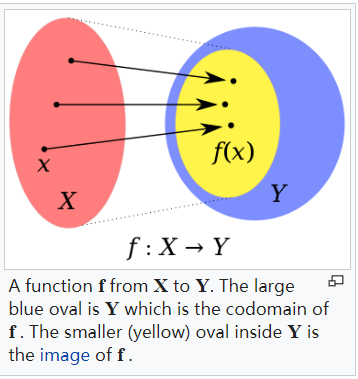
• For $ A : \mathcal{U} \to \mathcal{V} $
  • $ \mathsf{D}(A) := U $ the domain
  • $ \mathsf{N}(A) := \lbrace u \in \mathcal{U} \mid Au = 0 \rbrace $ the kernel
  • $ \mathsf{R}(A) := \lbrace f \in \mathcal{V} \mid f = Au, u \in \mathcal{U} \rbrace $ the range
• A is continuous at $ u \in \mathcal{U} $
  • if $ \forall ε > 0 \exists δ > 0 $ with
    $\lVert Au - Av \rVert_\mathcal{V} \leq ε \ \forall \ v\in \mathcal{U} \ \mathrm{with}\ \lVert u - v \rVert_\mathcal{U} \leq δ$
• $ A^* $ the (unique) adjoint operator of $ A $ with
  • $ \langle Au, v \rangle_\mathcal{V} = \langle u, A^*v \rangle_\mathcal{U} \ \forall \ u \in \mathcal{U}, v \in \mathcal{V} $
• For a subset $ \mathcal{X} \subset \mathcal{U} $, the orthogonal complement of $ \mathcal{X} $ is defined by
  • $ \mathcal{X}^\perp := \lbrace u \in \mathcal{U} \mid \langle u,v\rangle_\mathcal{U} = 0 \ \forall \ v \in \mathcal{X} \rbrace $
• Let $ A \in \mathcal{L}(\mathcal{U},\mathcal{V}) $. Then $ A $ is saide to be compact if for any bounded set $ B \subset \mathcal{U} $ the closure of its image $ \overline{A(B)} $ is compact in $ \mathcal{V} $. We denote the spave of compact operators by $ \mathcal{K}(\mathcal{U},\mathcal{V}) $.

Introduction

• Operator equations
  $Au = f$
  where $ A : \mathcal{U} \to \mathcal{V} $ is the forward operator acting between some spaces
  $ \mathcal{U} $ and $ \mathcal{V} $ , typically Hilbert or Banach Spaces
  $ f $ are the measured data
  $ u $ is the quantity we want to reconstruct from data

Well-Posed

• The well-posed problem if
  1. it has a solution $ \forall f \in \mathcal{V} $
  2. the solution is unique
  3. the solution depends continuously on the data i.e. small errors in the data f result in small errors in the reconstruction

Differentiation

• Evaluation the derivative of a function $ f \in L^2 [0, \pi /2 ] $
  $D f = f^\prime$
  where $ D : L^2 /[ 0, \pi /2 /] \to L^2 [ 0, \pi /2 ] $

• Prop The operator D is unbounded from $ L^2 /[ 0, \pi /2 /] \to L^2 [ 0, \pi /2 ] $

• Integral transform of the image:
  $f(x) = (Au) (x) := \int K(x,\xi) u(\xi) d\xi ,$
  $ u(\xi) $ is the “true” image
  $ K(x,\xi) $ is the point-spread function (PSF) which models the optics of the camera

Fatou lemma

Fatou’s lemma

Generalised Solutions

Orthogonal decomposition

• For $ A \in \mathcal{L}(\mathcal{U},\mathcal{V}) $, we have
  • $ \mathsf{R}^\perp(A) = \mathsf{N}(A^* ) $ then $ \overline{\mathsf{R}(A)} = \mathsf{N}(A^* )^\perp $
  • $ \mathsf{R}^\perp(A^* ) = \mathsf{N}(A) $ then $ \overline{\mathsf{R}(A^* )} = \mathsf{N}(A)^\perp $
• Hence, we can deduce the following orthogonal decompositions
  • $ \mathcal{U} = \mathsf{N}(A) \oplus \overline{\mathsf{R}(A^* )} $
  • $ \mathcal{V} = \mathsf{N}(A^* ) \oplus \overline{\mathsf{R}(A)} $
• Lemma 1. Let $ A \in \mathcal{L}(\mathcal{U},\mathcal{V}) $ . Then $ \overline{\mathsf{R}(A^* A)} = \overline{\mathsf{R}(A^* )} $

Minimal-norm Solutions

• An element $ u \in \mathcal{U} $ is called
  • a least-squares solution of $ Au =f $ if
    $\lVert Au - f \rVert_\mathcal{V} = inf\lbrace \lVert Av - f \rVert_\mathcal{V}, v \in \mathcal{U} \rbrace$
  • a minimal-norm solution of $ Au =f $ (and is denoted by $ u^\dagger $ ) if
    $ \lVert u^\dagger \rVert_\mathcal{U} \leq \lVert v \rVert_\mathcal{U} $ for all least squares solutions $ v $
• Thm 1. Let $ f \in \mathcal{V} \ \mathrm{and} \ A \in \mathcal{L}(\mathcal{U},\mathcal{V}) $. Then the following three assertions are equivalent
  1. $ u \in \mathcal{U} $ satisfies $ Au = P_{\overline{\mathsf{R}(A)}} f $
  2. $ u $ is a least squares solution of the inverse problem
  3. $ u $ solves the normal equation
     $A^* Au = A^* f$
• Thm 2. Let $ f \in \mathsf{R}(A) \oplus \mathsf{R}(A)^\perp $. Then there exists a unique minimal norm solution $ u^\dagger$ to the inverse problem and all least squares solutions are given by $ \lbrace u^\dagger \rbrace + \mathsf{N}(A) $

Decomposition of compact operators

• Thm 1. Let $ \mathcal{U} $ be a Hilbert space and $ A \in \mathcal{K}(\mathcal{U},\mathcal{U}) $ be self-adjoint. Then there exists an orthonormal basis $ \lbrace x_j \rbrace_{j\in\mathbb{N}} \subset \mathcal{U} \ \mathrm{of} \ \mathsf{R}(A) $ and a sequence of eigenvalues $ \lbrace \lambda_j \rbrace_{j\in\mathbb{N}} \subset \mathbb{R} $ with $ \lvert \lambda_1 \rvert \geq \lvert \lambda_2 \rvert \geq \cdots > 0 $ such that for all $ u \in \mathcal{U} $ we have
  $Au = \displaystyle \sum_{j=1}^{\infty} \lambda_j \langle u,x_j \rangle_\mathcal{U} x_j$
  The sequence $ \lbrace \lambda_j \rbrace_{j\in\mathbb{N}} $ is either finite or we have $ \lambda_j \to 0 $

Singular Value Decomposition

• the sequence $ \lbrace (\sigma_j, x_j, y_j) \rbrace $ is called singular system or singular value decomposition (SVD) of $ A $
• Let $ A \in \mathcal{K}(\mathcal{U},\mathcal{V}) $. Then there exists
  1. a not-necessarily infinite null sequence $ \lbrace \sigma_j \rbrace_{j\in\mathbb{N}} $ with $ \sigma_1 \geq \sigma_2 \geq \cdots > 0 $,
  2. an orthonormal basis $ \lbrace x_j \rbrace_{j\in\mathbb{N}} \subset \mathcal{U} \ \mathrm{of} \ \mathsf{N}(A)^\perp $,
  3. an orthonormal basis $ \lbrace y_j \rbrace_{j\in\mathbb{N}} \subset \mathcal{V} \ \mathrm{of} \ \overline{\mathsf{R}(A)} $ with
     $Ax_j = \sigma_j y_j, \ A^* y_j = \sigma_j x_j, \ \forall \ j \in \mathbb{N}$
     • For all $ u \in \mathcal{U} $ we have the representation
       $ Au = \displaystyle \sum_{j=1}^{\infty} \sigma_j \langle u,x_j \rangle y_j $
     • For the adjoint operator $ A^* $ we have the representation
       $ A^* f = \displaystyle \sum_{j=1}^{\infty} \sigma_j \langle f,y_j \rangle x_j \ \ \forall \ f\in \mathcal{V} $

Moore-Penrose inverse

• Let $ A \in \mathcal{L}(\mathcal{U},\mathcal{V}) $ and let $ \widetilde{A} := A\mid_{\mathsf{N}(A)^\perp} : \mathsf{N}(A)^\perp \to \mathsf{R}(A) $ denote the restriction of $ A $ to $ \mathsf{N}(A)^\perp $
  The Moore-Penrose inverse $ A^\dagger $ is defined as the unique linear extension of $ \widetilde{A}^{-1} $ to
  $\mathsf{D}(A^\dagger) = \mathsf{R}(A) \oplus \mathsf{R}(A)^\perp$
  with
  $\mathsf{N}(A^\dagger) = \mathsf{R}(A)^\perp$.

• Thm 1. Let $ A \in \mathcal{L}(\mathcal{U},\mathcal{V}) $. Then $ A ^\dagger $ is continuous, i.e. $ A ^\dagger \in \mathcal{L}(\mathsf{D},\mathcal{U}) $, if and only iff $ \mathsf{R}(A) $ is closed.

• Lemma 1. The MP inverse $ A^\dagger $ satisfies $ \mathsf{R}(A^\dagger) = \mathsf{N}(A)^\perp $ and the MP equations
  1. $ A A^\dagger A = A $ ,
  2. $ A^\dagger A A^\dagger = A^\dagger $,
  3. $ A^\dagger A = I - P_{\mathsf{N}(A)} $,
  4. $ A A^\dagger = P_{\overline{\mathsf{R}(A)}}\mid_{\mathsf{D}(A^\dagger)} $,
     where $ P_\mathsf{N} $ and $ P_\overline{\mathsf{R}} $ denote the orthogonal projections on $ \mathsf{N} \ \mathrm{and} \ \overline{\mathsf{R}} $, respectively

• Thm 2. For each $ f \in \mathsf{D}(A^\dagger) $, the minimal norm solution $ u^\dagger $ to the inverse problem is given via
  $u^\dagger = A^\dagger f$.

• Thm 3. Let $ A \in \mathcal{K}(\mathcal{U},\mathcal{V}) $ with an infinite dimensional range. Then, the MPi of $ A $ is discontinuous

• Thm 4. Let $ A \in \mathcal{K}(\mathcal{U},\mathcal{V}) $ with singular system $ \lbrace (\sigma_j, x_j, y_j) \rbrace_{j\in\mathbb{N}} $ and $ f \in \mathsf{D} (A^\dagger) $
  then the Moore-Penrose inverse of $ A $ can be written as
  $ A^\dagger f = \displaystyle \sum_{j = 1}^{\infty} \sigma_j^{-1} \langle f,y_j \rangle x_j $

  • The representation makes it clear that the inverse is unbounded. Indeed, taing the sequence $ y_j $ we note that $ \lVert A^\dagger y_j \rVert = \sigma_j^{-1} \to \infty $, although $ \lVert y_j \rVert = 1 $

Picard criterion

• We say that the data $ f $ satisfy the Picard criterion, if
  $\lVert A^\dagger f \rVert^2 = \displaystyle \sum_{j=1}^{\infty} \frac{\lvert \langle f,y_j \rangle \rvert^2}{\sigma_j^2} < \infty$

• Thm 1. Let $ A \in \mathcal{K}(\mathcal{U},\mathcal{V}) $ with singular system $ \lbrace (\sigma_j, x_j, y_j) \rbrace_{j \in \mathbb{N}} $, and $ f \in \overline{\mathsf{R}(A)} $. Then $ f \in \mathsf{R}(A) $ if and only if the Picard criterion is met

ill-posed

• An ill-posed inverse problem is mildly ill-posed if the singular values decay at most with polynomial speed, i.e. there exist $ \gamma, C > 0 $ such that $ \sigma_j \geq C j^{-\gamma} $ for all $ j $. We call the ill-posed inverse problem severely ill-posed if its singular values decay faster than with polynomial speed, i.e. for all $ \gamma, C > 0 $ one has that $ \sigma_j \leq C j^{-\gamma} $ for $ j $ sufficiently large.

Regularisation Theory

Since the Moore-Penrose inverse of $ A $ is unbounded

Variational Regularisation

The variation formulation of Tikhonov regularisation for some data $ f_\delta \in \mathcal{V} $
$\displaystyle\min_{u\in\mathcal{U}} \lVert Au - f_\delta \rVert^2 + \alpha\lVert u \rVert^2$
* fidelity function $ \mathcal{F}(Au,f) = \lVert Au - f_\delta \rVert^2 $
* regulariser $ \mathcal{J}(U) = \lVert u \rVert^2 $

the variational regularisation problem is
$\displaystyle\min_{u\in\mathcal{U}} \mathcal{F}(Au,f) + \alpha\mathcal{J}(U)$

Characteristic function

• Let $ \mathcal{C} \subset \mathcal{U} $ be a set.
  The function $ \mathcal{X}_\mathcal{C} : \mathcal{U} \to \overline{\mathbb{R}} $,
  $\displaystyle \mathcal{X}_\mathcal{C}(u) = {\begin{cases}0 &{\text{if }} u \in \mathcal{C},\\ \infty &{\text{if }} u \in \mathcal{U}\backslash \mathcal{C}\end{cases}}$
  is called the characteristic function of the set $ \mathcal{C} $
• The CF $ \mathcal{X}_\mathcal{C}(u) $ is convex iff $ \mathcal{C} $ is a convex set

Let $ E : \mathcal{U} \to \overline{\mathbb{R}} $ be a functional.

Proper

• A functional E is called proper if
  the effective domain dom(E) is not empty

Convex

• A functional E is called convex if
  $ E (\lambda u + (1 - \lambda) v) \leq \lambda E(u) + (1-\lambda) E(v) $
  for all $ \lambda \in (0,1) $ and all $ u,v \in dom(E) \ \mathrm{with} \ u \neq v $
• It is called strictly convex if the inequality is strict

Fenchel conjugat

• The functional E is called the Fenchel conjugate of E, such that
  $ E^* (p) = \displaystyle \sup_{u\in \mathcal{U}} \lbrace \langle p,u \rangle - E(u)\rbrace $
• For any functional $ E : \mathcal{U} \to \overline{\mathbb{R}} $ the following inequallity holds:
  $ E^{* * } := (E^* )^* \leq E $

Lower-semicontinuous l.s.c

• If E is proper, l.s.c and convex, then
  $ E^{* * } = E $

Subdifferential

• A functional E is called subdifferentiable at $ u \in \mathcal{U} $, if there exists an element $ p \in \mathcal{U}^* $ such that
  $ E(v) \geq E(u) + <p,v-u> \ \forall v \in \mathcal{U} $
• $ p $ also called a subgradient at position $ u $
• the collection of all subgradients at position $ u $ is called subdifferential of $ E $ at $ u $, such that
  $ \partial E(u) := \lbrace p \in \mathcal{U}^* \mid E(v) \geq E(u) + <p, v-u>, \ \forall v \in \mathcal{U} \rbrace $

Minimiser

• We call $ u^* $ a minimiser of $ E $ such that
  $ u^* \in \mathcal{U} $ solves the minimisation problem $ \displaystyle \min_{u \in \mathcal{U}} E (u) $
  if and only if $ E(u^* ) \leq \infty $ and $ E(u^* ) \leq E(u), \ \forall u \in \mathcal{U} $
• An element $ u \in \mathcal{U} $ is a minimiser of $ E $ if and only if $ 0 \in \partial E(u) $

Weak compact convex subset 4.1.19

• Let $ E $ be a proper convex fucntion and $ u \in \ \mathrm{dom} \ (E) $ . Then $ \partial E(u) $ is a weak-* compact convex subset of $ \mathcal{U}^* $ .

Bregman distances

• Let $ E $ be a convex functional. Moreover, let $ u,v \in \mathcal{U}, \ E(v) \leq \infty \ \mathrm{and} \ q \in \partial E(v) $. Then the (generalised) Bregman distance of $ E $ between $ u $ and $ v $ is defined as
  $D^q_E(u,v):= E(u) - E(v) - <q,u-v>$.

In general, the Bregman distances are not symmetric that $ D^q_E (u,v) = 0 $ does not imply $ u =v $, overcome the issue, one can introduce the symmetric Bregman distance

• Let $ E $ be a convex functional. Moreover, let $ u,v \in \mathcal{U}, \ E(u) \leq \infty, E(v) \leq \infty \ \mathrm{and} \ q \in \partial E(v) $. Then the symmetric Bregman distance of $ E $ between $ u $ and $ v $ is defined as
  $D^\mathrm{symm}_E(u,v):= D^q_E(u,v) + D^p_E(v,u) = <p-q,u-v>$.

Absolutely one-homogeneous functionals

• A functional $ E $ is called absolutely one-homogeneous if
  $E(\lambda u) = \lvert \lambda \rvert E(u) \ \forall \ \lambda \in \mathbb{R}, \ \forall \ u\in\mathcal{U}$
• Prop 1. Let $ E(\cdot) $ be a convex absolutely one-homogeneous functional and let $ p \in \partial E(u) $. Then the following equality holds:
  $E(u) = (p,u)$.
• Prop 2. Let $ E(\dot) $ be a proper, convex, l.s.c. and absolutely one-homogeneous functional. Then the Fenchel conjugate $ E^* (\cdot) $ is the characteristic function of the convex set $ \partial E(0) $.
• Prop 3. For any $ u \in \mathcal{U}, p \in \partial E(u) $ if and only if $ p \in \partial E(0) $ and $ E (u) = (p,u) $.

Coercive

• A functional E is called coercive, if for all $ \lbrace u_j \rbrace_{j\in \mathbb{N}} $ with $ \lVert u_j \rVert_\mathcal{U} \to \infty $ we have $ E(u_j) \to \infty $

Level set

• $ L_c (f) = \lbrace (x_1, \cdots, x_n ) \mid f(x_1 , \cdots x_n ) = c \rbrace $
• Sub-level set of f is
  • $ L_c^- (f) = \lbrace (x_1, \cdots, x_n ) \mid f(x_1 , \cdots x_n ) \leq c \rbrace $

J-minimising solutions

• Suppose that the fidelity term is such that the optimisation problem
  $\displaystyle\min_{u\in\mathcal{U}} \mathcal{F}(Au,f)$
  has a solution for any $ f \in \mathcal{V} $. Let
  • $ u^\dagger_\mathcal{J} \in \arg \min_{u\in\mathcal{U}} \mathcal{F}(Au,f) $ and
  • $ \mathcal{J}(u^\dagger_\mathcal{J})\leq \mathcal{J}(\tilde{u})\ \forall \ \tilde{u}\in \arg \min_{u\in\mathcal{U}}\mathcal{F}(Au,f) $
    Then $ u^\dagger_\mathcal{J} $ is called a $ \mathcal{J} $ -minimising solution of $ Au = f $

Main result of well-posedness

• Let $ \mathcal{U} $ and $ \mathcal{V} $ be Banach spaces and $ \tau_\mathcal{U} $ and $ \tau_\mathcal{V} $ some topologies (not necessarily induced by the norm) in $ \mathcal{U} $ and $ \mathcal{V} $, respectively. Suppose that problem $ Au = f $ is solvable and the solution has a finite value of $ \mathcal{J} $. Assume also that
  1. $ A : \mathcal{U} \to \mathcal{V} $ is $ \tau_\mathcal{U} \to \tau_\mathcal{V} $ continuous;
  2. $ \mathcal{J}: \mathcal{U} \to \overline{\mathbb{R_+}} $ is proper, $ \tau_\mathcal{U} $ -l.s.c and its non-empty sublevel-sets $ \lbrace u \in \mathcal{U} : \mathcal{J}(u) \leq C \rbrace $ are $ \tau_\mathcal{U} $ -sequentiallly compact;
  3. $ \mathcal{F}: \mathcal{V} \times \mathcal{V} \to \overline{\mathbb{R_+}} $ is proper, $ \tau_\mathcal{V} $ -l.s.c in the first argument and norm-l.s.c in the second ne and satisfies
     $\mathcal{F}(f,f) = 0 \ \mathrm{and} \ \mathcal{F}(f,f_\delta) \leq C(\delta) \to 0 \ \mathrm{as}\ \delta \to 0$
     $ \ \forall \ f\in \mathcal{V} \ \mathrm{and} \ f_\delta \in \mathcal{V} \ \mathrm{s.t.} \ \lVert f_\delta - f \rVert \leq \delta $ ;
  4. there exists an a priori parameter choice rule $ \alpha = \alpha(\delta) $ such that $ \displaystyle \lim_{\delta\to 0} \alpha(\delta) = 0 \ \mathrm{and} \ \displaystyle \lim_{\delta\to0} \frac{C(\delta)}{\alpha(\delta)} = 0 $

  Then

  i. there exists a $ \mathcal{J} $ -minimising solution $ u^\dagger_\mathcal{J} $ of $ Au=f $;
  ii. for any fixed $ \alpha > 0 $ and $ f_\delta \in \mathcal{V} $ there exists a minimiser $ u^\alpha_\delta \in \arg \min_{u\in\mathcal{U}} \mathcal{F}(Au,f_\delta) + \alpha\mathcal{J}(u) $;
  iii. the parameter choice rule $ \alpha = \alpha(\delta) $ from Assumption(4) guarantees that $ u_\delta := u^{\alpha(\delta)}_ \delta \xrightarrow[]{\tau_\mathcal{U}} u^\dagger_\mathcal{J} $ (possibble, along a subsequence) and $ \mathcal{J}(u_\delta) \to \mathcal{J}(u^\dagger_\mathcal{J}) $

Total Variation Regularisation

• Let $ \Omega \subset \mathbb{R}^n $ be a bounded domain and $ u \in L^1(\Omega) $. Let $ \mathcal{D}(\Omega, \mathbb{R}^n) $ be the following set of vector-valued test function (i.e. functions that map from $ \Omega $ to $ \mathbb{R}^n $)
  $\mathcal{D} (\Omega,\mathbb{R}^n) := \lbrace \varphi \in C^\infty_0 (\Omega;\mathbb{R}^n) \mid \ \mathrm{ess} \ \sup_{x\in\Omega} \lVert \varphi(x) \rVert_2 \leq 1 \rbrace$.
• total variation of $ u \in L^1(\Omega) $ is defined as follows
  $\ \mathrm{TV} \ (u) \displaystyle \sup_{\varphi\in\mathcal{D}(\Omega,\mathbb{R}^n)} \int_{\Omega} u(x) \ \mathrm{div} \ \varphi(x) dx$

Dual Perspective

Numerical Optimisation Methods

Example

Topics in Convex Optimisation

Numerical Solution of Differential Equations

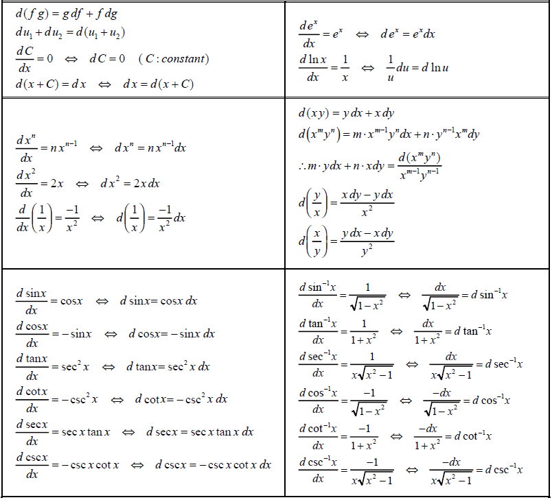
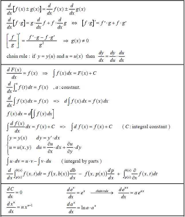
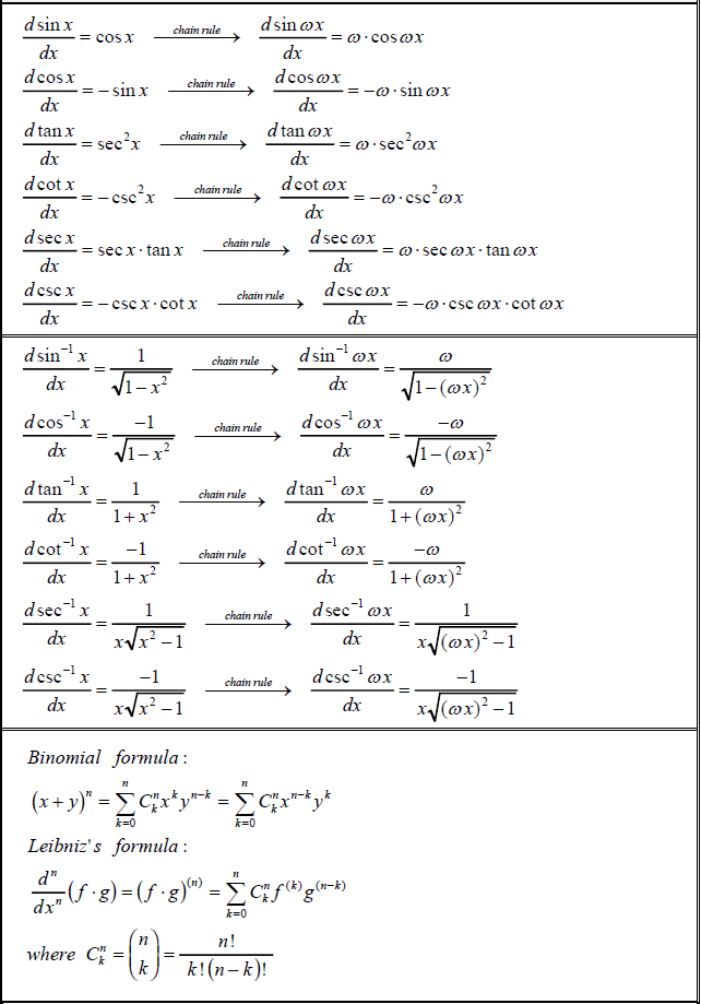
Calculus

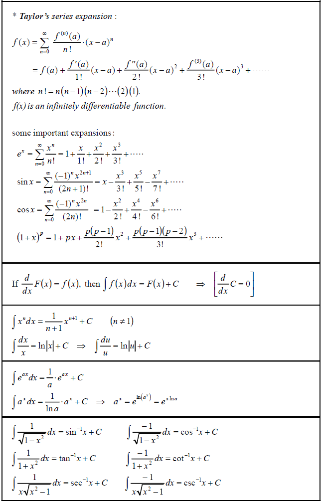
Series Expansion

Complex exponential formula
$ \sin(x) = \displaystyle \frac{e^{ix}-e^{-ix}}{2i} $
$ \cos(x) = \displaystyle \frac{e^{ix}+e^{-ix}}{2} $
hyperbolic function: $ \sinh(x) = -i \sin(ix) \; \cdots $