
These are the notes by learning the “Introduction to Probability and Data” from Coursera.org for future reviews.
Introduction to Data
- Data matrix: data are organized in
- Observation (case): row
- Variable: column
Types of variables
- Numerical
- numerical values (sensible to add, subtract, take averages, etc. with them) 1. continuous: infinite number of values within a given range 2. discrete: specific set of numeric values
- Categorical
- limited number of distinct categories (not sensible to do arithmetic operations)
- ordinal: inherent ordering
- Nominal: not ordering
- limited number of distinct categories (not sensible to do arithmetic operations)
Relationships between variables
- associated (dependent) : positive or negative
- independent : not associated
Observational study
- collect data in a way that does not directly interfere with how data arise (“observe”)
- only establish an association
- retrospective: use past data
- prospective: data are collected throughout the study
Experiment study
- randomly assign subjects to treatments
- establish causal connections
Why not Census
- some individuals are hard to locate or measure, and these people be different from the rest of the population
- populations rarely stand still
Sources of Sampling bias
- Convenience sample: individuals who are easily accessible are more likely to be included in the sample
- Non-response: If only a (non-random) fraction of the randomly sampled people respond to survey such that the sample is no longer representative of the population
- Voluntary response: Occurs when the sample consists of people who volunteer to respond because they have strong opinions on the issue
Sample Methods
- simple random sampling: randomly select cases from the population
- stratified sampling: first divide the population into homogenous groups called strata, and then randomly sample from within each stratum
- cluster sampling: divide the population into clusters, randomly sample a few clusters, and then sample all observation within these clusters
- multistage sampling: divide the population into clusters, randomly sample a few clusters, and then we randomly sample observations from within these clusters
Experimental design
- Principles of Experimental Design:
- control: compare treatment of interest to a control group
- randomize: randomly assigning subjects to treatments
- replicate: collect a sufficiently large sample, or replicate the entire study
- block: block for variables known or suspected to affect the outcome
- confounding variable: is correlated with both the explanatory and response variables
- Explanatory variables (factors): conditions we can impose on our experimental units
- Blocking variables: characteristics that the experimental units come with, that we would like to control for
- Blocking is like stratifying:
- blocking during random assignment
- stratifying during random sampling
Experimental terminology
- placebo: fake treatment, often used as the control group for medical studies
- placebo effect: showing change despite being on the placebo
- blinding: experimental units do not know which group they are in
- double-blind: both the experimental units and the researchers do not know the group assignment
Random sampling and random assignment
| ideal experiment $\searrow$ | Random Assignment | No Random Assignment | most observational studies $\swarrow$ |
| Random Sampling | Causal and Generalizable | not Causal, but Generalizable | Generalizability |
| No Random Sampling | Causal, but not Generalizable | neither Causal nor Generalizable | Np Generalizability |
| most experiments $\nearrow$ | Causation | Association | bad observational studies $\nwarrow$ |
Exploratory Data Analysis and Introduction to Inference
Scatterplots
- explanatory variable on x axis
- response variable on y axis
- correlation, not causation
Evaluate the relationship
- direction: positive or negative
- shape: linear or curved or others
- strength: strong or weak
- outliers
Histogram
- provide a view of the data density
- especially useful for identifying shapes of distributions
Skewness
- distributions are skewed to the side of the long tail
- left skewed: the longer tail is on the left on the negative end
- mean < median
- symmetric: no skewness is apparent
- mean $\approx$ median
- right skewed: the longer tail is on the right, the positive end
- mean > median
- left skewed: the longer tail is on the left on the negative end
Modality
- unimodal: one prominent peak (normal distribution or bell curve)
- bimodal: two prominent peak (might two distinct groups in data)
- uniform: no prominent peaks (no apparent trend)
- multimodal: more than two prominent peaks
Bin width
the chosen bin width can alter the story the histogram is telling
- bin width too wide: might lose interesting details
- bin width too narrow: might be difficult to get an overall picture of the distribution
- ideal bin width depends on the data you are working with
Dot plot
- useful when individual values are of interest
- can get too busy as the sample size increases
Box plot
- useful for highlighting outliers, media, IQR(interquartile range)
Intensity map
- useful for highlighting the spatial distribution
Measures of spread
- range: (max - min)
- variance: roughly the average squared deviation from the mean
- sample variance: $s^2$
- population variance: $(\sigma)^2$
- $s^2 = \frac{\sum_{i=1}^{n} (x_i - \bar{x})^2}{n-1}$
- standard deviation: roughly the average deviation around the mean, and has the same units as the data
- sample sd: $s$
- population sd: $\sigma$
- inter-quartile range
- range of the middle 50% of the data, distance between the first quartile (25th percentile) and third quartile (the 75th percentile)
- most readily available in a box plot.
- $IQR = Q_3 - Q_1$
Robust Statistics
- define: measures on which extreme observations have little effect
- robust measures of center & spread:
| robust | non-robust | |
|---|---|---|
| center | median | mean |
| spread | IQR | SD, range |
Transforming data
- define: a rescaling of the data using a function
- When data are very strongly skewed, we sometimes transform them, so that they are easier to model
- (natural) log transformation:
- often applied when much of the data cluster near zero (relative to larger values in the dataset) and all observations are positive
- to make the relationship between the variables more linear, and hence easier to model with simple methods
- other transformations:
- square root
- inverse
- goals:
- to see the data structure differently
- to reduce skew assist in modeling
- to straighten a nonlinear relationship in a scatterplot
Exploring Categorical Variables
- Bar plots
- Q: How are bar plots different than histograms?
- barplots for categorical variables, histograms for numerical variables
- x-axis on a histogram is a number line, and the ordering od the bars are not interchangeable
- Segmented bar plot
- useful for visualizing conditional frequency distributions
- compare relative frequencies to explore the relationship between the variables
- Relative frequency segmented bar plot
- Mosaicplot
- Side-by-side box plots
Introduction to inference
- null hypothesis($H_0$): independent, “There is nothing going on”
-
alternative hypothesis($H_A$): dependent, “There is something going on”
- hypothesis testing framework
- start with a null hypothesis($H_0$) that represents that status quo
- set an alternative hypothesis($H_A$) that represents our research question, i.e. what we’re testing for
- conduct a hypothesis test under the assumption that the null hypothesis is true, either via simulation or using theoretical methods
- If the test results suggest that the data do not provide convincing evidence for the alternative hypothesis, we stick with the null hypothesis
- If they do, then we reject the null hypothesis in favor of the alternative
Inference summary
- set a null and an alternative hypothesis
- simulate the experiment assuming that the null hypothesis is true
- evaluated the p_value: probability of observing an outcome at least as extreme as the one observed in the original data
- if this probability is low, reject the null hypothesis in favor of the alternative
Probability and Distribution
-
random process: know what outcomes could happen, but don’t know which particular outcome will happen
- P (A) = Probability of event A
- 0≤P(A)≤1
-
frequentist interpretation: The probability of an outcome would occur if we observed the random process an infinite number of times.
-
Bayesian interpretation: A Bayesian interprets probability as a subjective degree of belief
-
largely popularized by revolutionary advance in computational technology and methods during the last twenty years
-
law of large members: sates that as more observations are collected, the proportion of occurrences with a particular outcome converges to the probably of that outcome
-
common misunderstanding: gambler’s fallacy (law of averages)
- disjoint (mortally exclusive) events cannot happen at the same time
- P(A & B) = 0
- Union of disjoint events: P(A or B) = P(A) + P(B) - P(A & B)
- Complementary → disjoint; complementary !← disjoint
- non-disjoint events can happen at the same time
- P(A & B) != 0
-
sample space: a collection of all possible outcomes of a trial
-
probability distribution: all possibility outcomes in the sample space, and the probabilities with they occur
- Rules:
- the events listed must be disjoint
- each probability must be between 0 and I
- the probabilities must total I
- complementary events: two mentally exclusive events whose probabilities add up to l
-
Independence: P(A/B) = P(A), P(A1, … & Ak<\sub>) = P(A1) × … × P(Ak)
-
Dependence: P(A/B) = P(A & B)/ P(B), P(A & B) = P(A/B) × P(B)
-
Posterior Probability: P(hypothesis / data) → P(hypothesis is true / observed data)
- P-value: P(data / hypothesis) → P(observed or more extreme outcome / H0 is true)
Normal Distribution
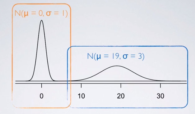
Normal distribution $N( \mu , \sigma )$
- unimodal and symmetric
- bell curve
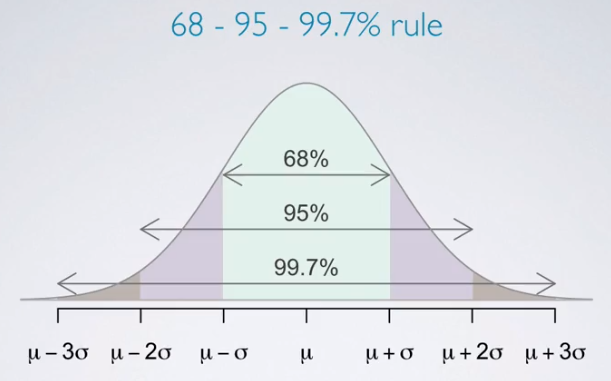
- follows very strict guidelines about how variably the data are distributed around the mean
- Many variables are nearly normal, but none are exactly normal
- two parameters: mean μ and stand deviation σ
- Changing the center and the spread of the distribution changes the overall shape of the distribution
- rules govern the variability of normally distributed data around the mean
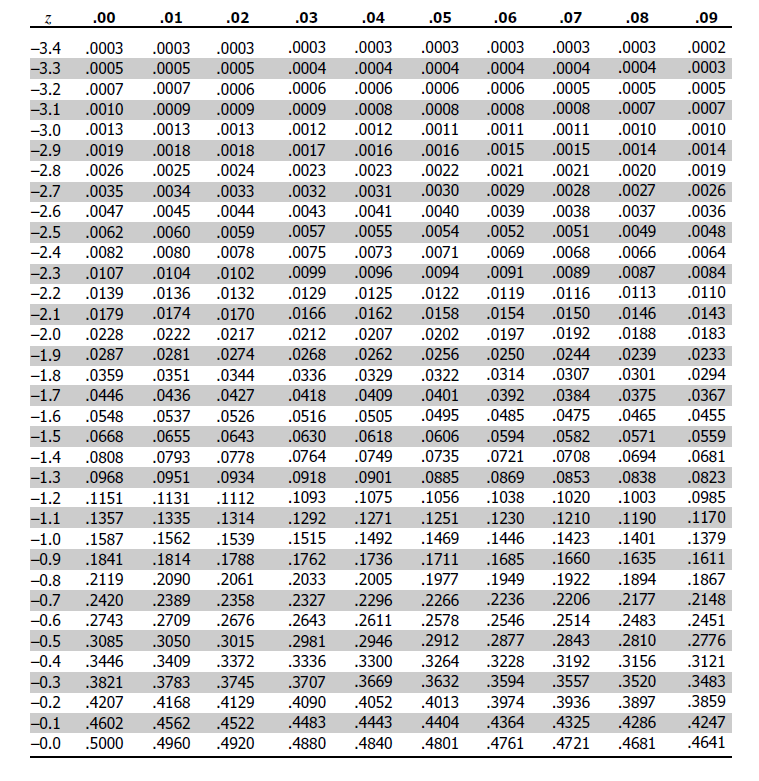
Standardizing with Z scores
- standardized (Z) score of an obervation is the number of standard deviations it falls above or below the mean
- $Z = \frac{observation - mean}{SD}$
- Z score of mean = 0 (normally: median ≈ 0 )
- unusual observation: $\lvert Z\rvert > 2$
- defined for distributions of any shape
- when the distribution is normal, Z scores can be used to calculate percentiles
- Percentile is the percentage of observations that fall below a given data point
- graphically, percentile is the area below the probability distribution curve to the left of that observation
- if the distribution does not follow the nice unimodal symmetric normal shape, you’d need to use calculus for that
- Methods for Z scores
- Using R: pnorm(-1, mean = 0, sd = 1) (qnorm for quantiles or cutoff values)
- Distribution Calculator
- Table
Evaluating
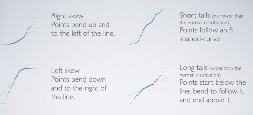
- anatomy of a normal probability plot
- Data are plotted on the y-axis of a normal probability plot, and theoretical quantiles (following a normal distribution) on the x-axis
- If there is a one-to-one relationship between the data and the theoretical quantiles, then the data follow a nearly normal distribution.
- Since a one-to-one relationship would appear as a straight line on a scatter plot, the closer the points are to a perfect straight line, the more confident we can be that the data follow a normal model.
- Constructing a normal probability plot requires calculating percentiles and corresponding z-scores for each observation, which is tedious. Therefore, we generally rely on software when making these plots.
- Also can using 68-95-99.7% rule
Binomial Distribution
- binomial distribution describes the probability of having exactly k successes in n independent Bernoulli trials with probability of success p
- # of scenarios × P(single scenario)
- $P(k = K) = {n \choose k} p^k (1-p)^{(n-k)}$
in R: dbinom(k, size, p) Distribution Calculator
- Choose function: ${n \choose k}=\dfrac{n!}{k!(n−k)!}$
in R: choose(n, k)
Binomial conditions
- The trials are independent.
- The number of trials, n, is fixed.
- Each trial outcome can be classified as a success or failure.
- The probability of a success, p, is the same for each trial.
- Expected value (mean) of binomial distribution ($\mu = np$) and its standard deviation ($\sigma = \sqrt{np(1-p)}$)
normal approximation
-
Fact: when the number of trials increases, the shape of the binomial actually starts looking closer and closer to a full normal distribution
- Calculate the probabilities for each outcome from a to b and sum them up
in R: sum(dbinom(a:b, size = n, p =p))
- Success-failure rule: a binomial distribution with at least 10 expected successes and 10 expected failures closely follows a normal distribution
- $np \geq 10$
- $n( 1-p ) \geq 10$
- Normal approximation to the binomial: If the success-failure condition holds, then
- $ Binomial(n,p) \thicksim Normal(\mu,\sigma) $
- where $ \mu = np $ and $ \sigma = \sqrt{np(1-p)} $